Functions 'bottom left', 'top left', 'bottom right', and 'top right' named by their initials, provide very low level relative positional structures for use in raster logic. These are used to traverse the divide left by area-based rasters which are inherently a discrete value across a finite element. If we want that element as part of a continuous surface we need to find local relative values for its corners. Used in quadmesh and anglr packages, and useful for calculating neighbourhood values.
bl(x)

tl(x)

br(x)

tr(x)

image0(x, ...)

image1(x, ...)

text0(x, ...)
Arguments
| x | matrix |
|---|---|
| ... | arguments passed to image() |
Value
matrix, padded by one row and one column relative to input
Details
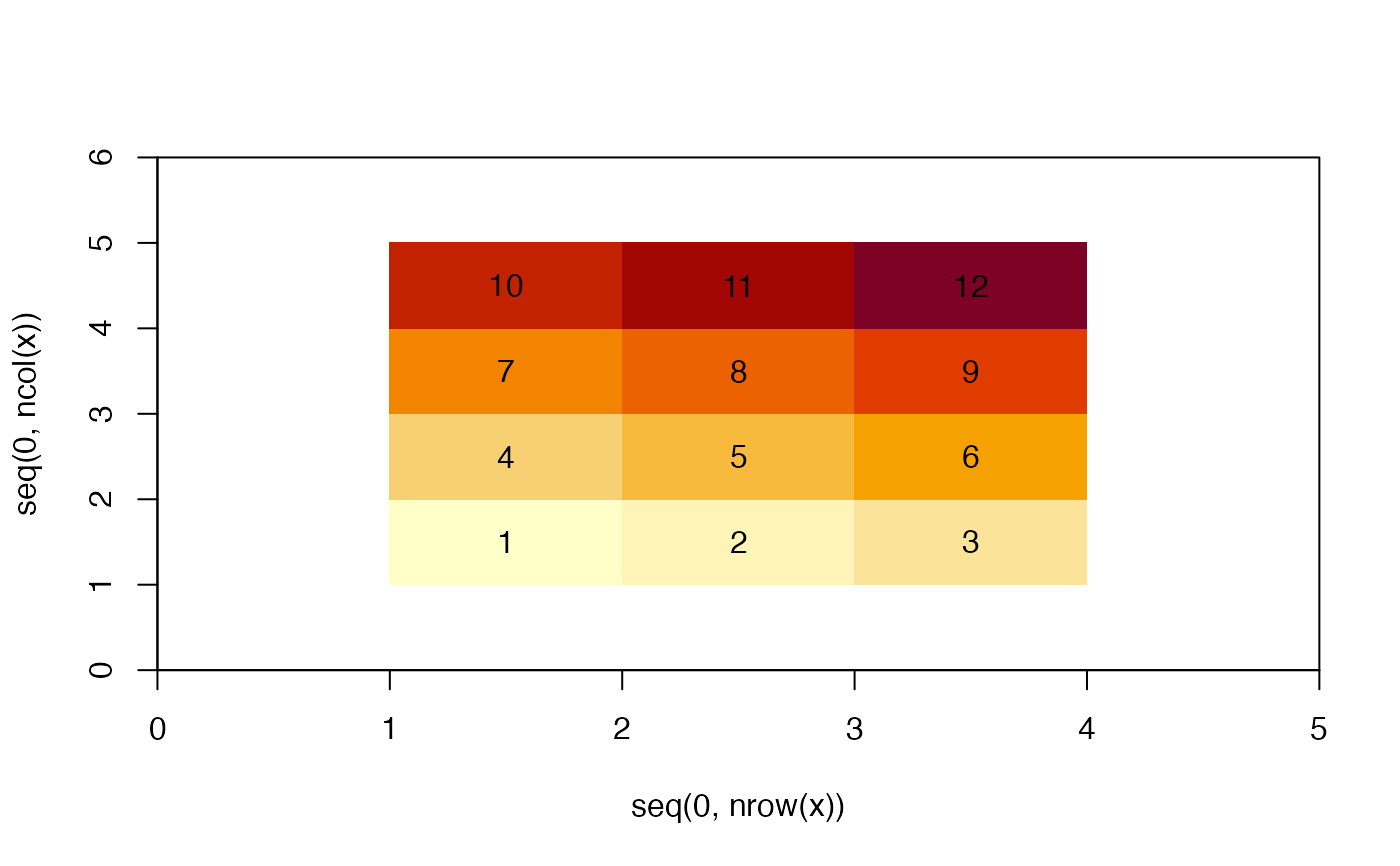
Some tiny functions 'image0', 'image1', 'text0' exist purely to illustrate the ideas in a vignette.
Examples
#> [,1] [,2] [,3] [,4] #> [1,] 1 4 7 10 #> [2,] 2 5 8 11 #> [3,] 3 6 9 12tl(m)#> [,1] [,2] [,3] [,4] [,5] #> [1,] NA 1 4 7 10 #> [2,] NA 2 5 8 11 #> [3,] NA 3 6 9 12 #> [4,] NA NA NA NA NAtr(m)#> [,1] [,2] [,3] [,4] [,5] #> [1,] 1 4 7 10 NA #> [2,] 2 5 8 11 NA #> [3,] 3 6 9 12 NA #> [4,] NA NA NA NA NAbl(m)#> [,1] [,2] [,3] [,4] [,5] #> [1,] NA NA NA NA NA #> [2,] NA 1 4 7 10 #> [3,] NA 2 5 8 11 #> [4,] NA 3 6 9 12br(m)#> [,1] [,2] [,3] [,4] [,5] #> [1,] NA NA NA NA NA #> [2,] 1 4 7 10 NA #> [3,] 2 5 8 11 NA #> [4,] 3 6 9 12 NAtl(br(m))#> [,1] [,2] [,3] [,4] [,5] [,6] #> [1,] NA NA NA NA NA NA #> [2,] NA 1 4 7 10 NA #> [3,] NA 2 5 8 11 NA #> [4,] NA 3 6 9 12 NA #> [5,] NA NA NA NA NA NAimage0(tl(br(m)))text0(tl(br(m)))