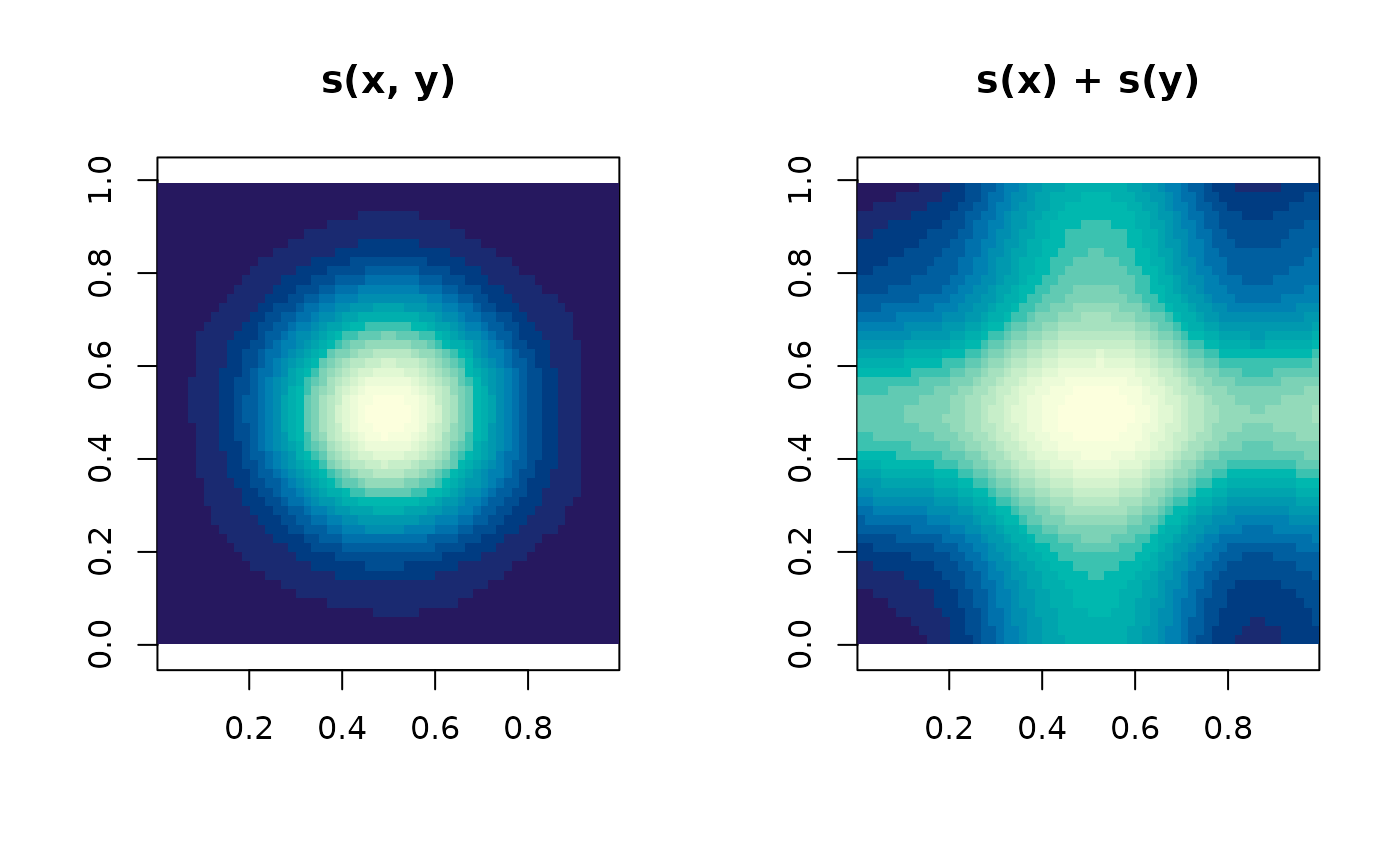
Generalized additive model on the coordinates

Fit a smooth of x and y with mgcv::gam() and predict it at every cell.

Usage

grid_gam(
  x,
  value = NULL,
  grid = NULL,
  formula = value ~ s(x, y),
  statistic = c("prediction", "se"),
  ...
)

Arguments

x: coordinates, or coordinates carrying their value as z; see xyz_input()
value: one value per coordinate, or NULL to use the z of x
grid: a grid_spec() to interpolate onto, or NULL for a default one
formula: a model formula in value, x and y
statistic: "prediction" for the fitted surface, "se" for its standard error
...: passed to mgcv::gam()

Value

A guerrilla_grid with values.

Details

The default formula is value ~ s(x, y), one isotropic two dimensional smooth. That matters: mgcv's default basis for a two dimensional s() is a thin plate regression spline, so this is grid_tps() with the number of basis functions reduced and the smoothing parameter chosen by REML. The two give visibly similar surfaces on the same data, and seeing that is worth more than either surface on its own.

value ~ s(x) + s(y) is the wrong model for a surface and a useful thing to try: additive in x and y means every column of the grid has the same shape as every other, so it cannot represent a feature that sits in one place. Pass it as formula and look.

Examples

xy <- cbind(runif(200), runif(200))
v <- exp(-20 * ((xy[, 1] - 0.5)^2 + (xy[, 2] - 0.5)^2))
if (requireNamespace("mgcv", quietly = TRUE)) {
  op <- par(mfrow = c(1, 2))
  plot(grid_gam(xy, v), main = "s(x, y)")
  ## additive in x and y cannot put a bump in one place
  plot(grid_gam(xy, v, formula = value ~ s(x) + s(y)), main = "s(x) + s(y)")
  par(op)
}