Triangles, tiles, and the weights between them

Michael D. Sumner

2026-09-09

Two of the methods in this package come from tessellating the plane rather than fitting anything: cut the space up around the data points, then let each piece answer for the region it covers. They give the two simplest honest answers there are, and the arithmetic behind both fits on one page.

library(guerrilla)
library(readxl)
bw <- read_excel(system.file("extdata", "BW-Zooplankton_env.xls",
                             package = "guerrilla", mustWork = TRUE))
lonlat <- as.matrix(bw[, c("Lon", "Lat")])
val <- bw$temp
g <- grid_spec(lonlat, crs = "EPSG:4326")

The two tessellations

GEOS builds both, and they are duals of each other.

library(geos)
pts <- as_geos_geometry(wk::xy(lonlat[, 1], lonlat[, 2]))
coll <- geos_make_collection(pts)

op <- par(mfrow = c(2, 1), mar = c(2, 2, 2, 1))
plot(geos_unnest(geos_delaunay_triangles(coll), keep_multi = FALSE),
     col = NA, border = "grey40", main = "Delaunay triangles")
points(lonlat, pch = 16, cex = 0.4)
plot(geos_unnest(geos_voronoi_polygons(coll), keep_multi = FALSE),
     col = NA, border = "grey40", main = "Voronoi tiles")
points(lonlat, pch = 16, cex = 0.4)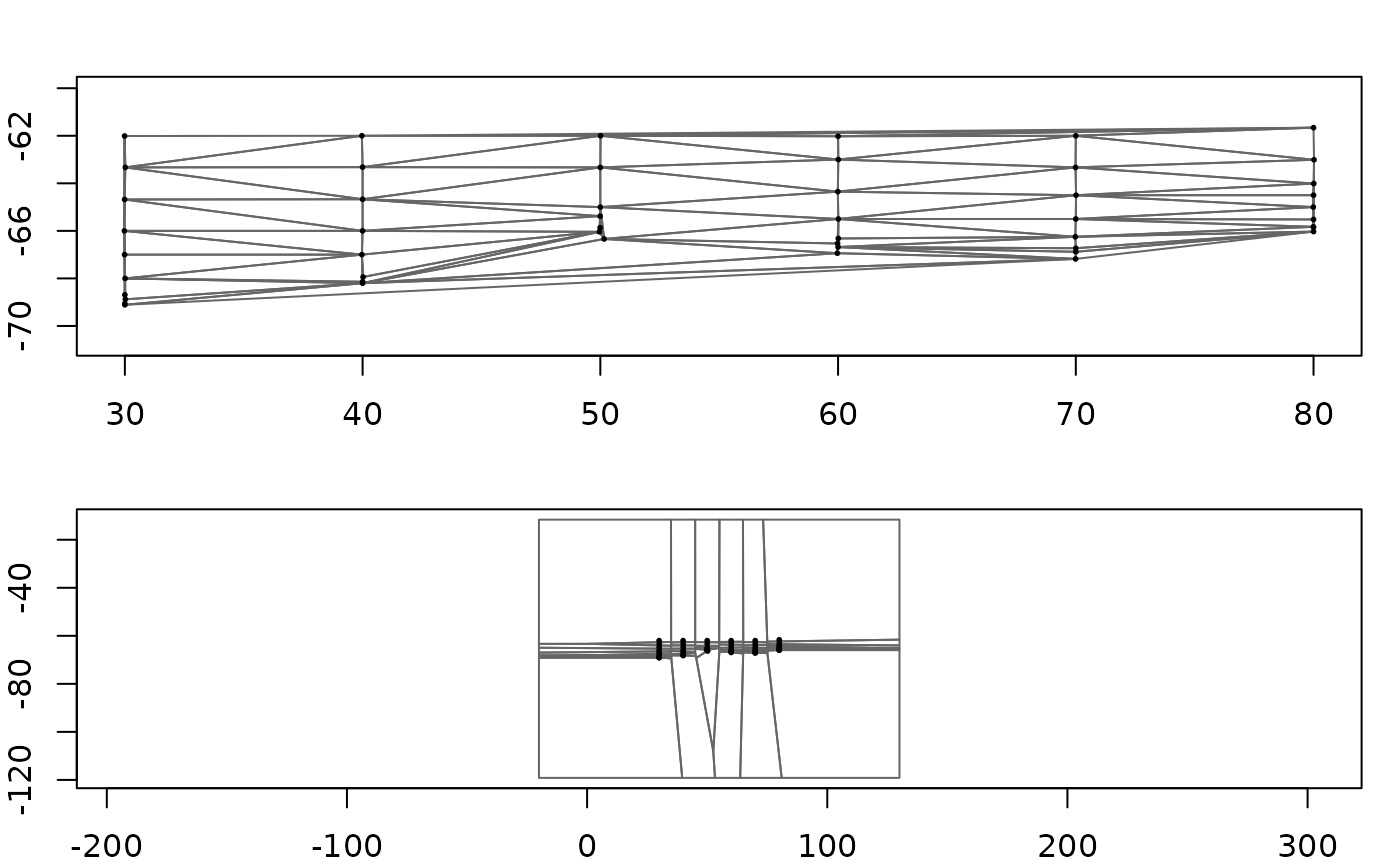

par(op)

They answer different questions. A Delaunay triangle has three data points at its corners, so a value inside it can be a blend of three. A Voronoi tile has one data point in it and consists of everywhere closer to that point than to any other, so a value inside it can only be that one point’s value.

Which means the Voronoi tessellation is nearest neighbour:

plot(grid_voronoi(lonlat, val, g))
points(lonlat, pch = 16, cex = 0.3)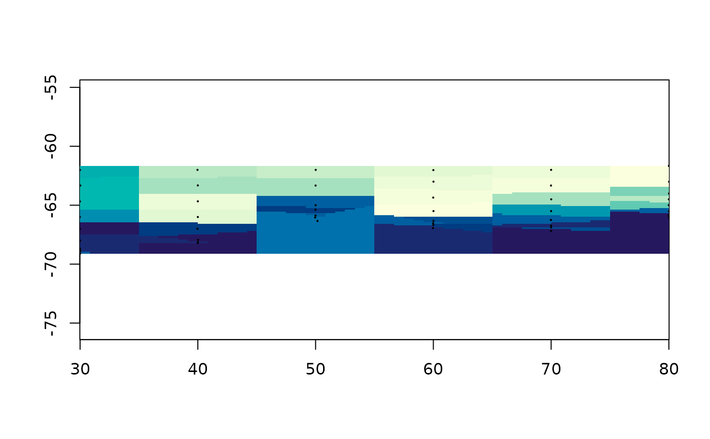

Barycentric coordinates

The Delaunay case needs one idea. For a point inside a triangle, the barycentric weights say how much of each corner the point is made of. They sum to one, and they are all non-negative exactly when the point is inside – so the same three numbers are both a point-in-triangle test and the interpolation rule.

tri <- cbind(c(0, 1, 0), c(0, 0, 1))
bary_weights(tri, rbind(c(0.25, 0.25), c(1/3, 1/3), c(1, 1)))
#>            [,1]      [,2]      [,3]
#> [1,]  0.5000000 0.2500000 0.2500000
#> [2,]  0.3333333 0.3333333 0.3333333
#> [3,] -1.0000000 1.0000000 1.0000000

The first point is a quarter of the way in from two corners; the second is the centroid, made equally of all three; the third is outside, which shows up as a negative weight rather than as a separate test.

The whole of bary_weights() is Cramer’s rule on a two by two system, six lines of arithmetic. Reading it is a better use of ten minutes than reading any description of it, including this one.

Interpolating is then the weighted sum of the corner values:

tri_grid <- grid_barycentric(lonlat, val, g)
plot(tri_grid)

Inside each triangle the surface is the plane through its three corner values, so the result is continuous, passes exactly through the data, and invents nothing beyond it. Cells outside the convex hull are in no triangle and stay NA – unlike the Voronoi fill above, which covers everything. That is convenient, and it is also nearest neighbour’s main way of lying to you: a cell far from any data still gets a confident answer.

Two engines, one answer

grid_barycentric() normally gets its result from one call to geometry::tsearch(), which finds the containing triangle for every cell and its weights in a single pass of C. That is the right way to compute it and the wrong way to learn it, so the same job is also written out in R: find_triangle() to locate each cell, bary_weights() to weight it.

slow <- grid_barycentric(lonlat, val, g, engine = "R")
ok <- !is.na(slow$values)
max(abs(slow$values[ok] - tri_grid$values[ok]))
#> [1] 6.605827e-15

The readable one is much slower and agrees to floating point. It is not there for speed, it is there so the claim “this is what the C is doing” can be checked rather than believed.

find_triangle() is worth a look on its own, because the search is the part people assume is hard. It asks GEOS which triangles a point could be in, using an STRtree index, then uses bary_weights() to decide which one it actually is.

triangles <- geometry::delaunayn(lonlat)
find_triangle(lonlat, triangles, rbind(c(50, -65), c(0, 0)))
#> [1] 51 NA

The second point is nowhere near the data, and gets NA.

The long way round, and a bug it revealed

Three points determine a plane, and least squares through exactly three points is that plane. So fitting value ~ x + y inside each Delaunay triangle must give the same surface as barycentric interpolation:

lm_grid <- grid_facet_lm(lonlat, val, g)
both <- !is.na(lm_grid$values) & !is.na(tri_grid$values)
max(abs(lm_grid$values[both] - tri_grid$values[both]))
#> [1] 5.417888e-14

It does, and it is enormously slower, and seeing that happen once is worth the wait.

This package used to offer that as facets(), with a Dirichlet variant alongside the Delaunay one. The Dirichlet variant was not doing what it looked like it was doing. A Voronoi tile holds exactly one point, so the per-tile lm(value ~ x + y) had one observation and three parameters. It fitted an intercept, predicted that single value across the whole tile, and produced – bit for bit – nearest neighbour, computed by running a linear model per tile in an R loop.

Brute force nearest neighbour, one line, gives exactly the same numbers:

at <- grid_xy(g)
nearest <- apply(at, 1, function(p) which.min((lonlat[, 1] - p[1])^2 +
                                              (lonlat[, 2] - p[2])^2))
identical(grid_voronoi(lonlat, val, g)$values, val[nearest])
#> [1] TRUE

facets() is still exported and still works, marked superseded. The lesson is not that it was slow. It is that a method can be named after its machinery rather than its answer, and then nobody notices for years what answer it gives. Every function added in this package is named for what it computes, because of this one.

The same thing, from a mesh

A grid is one particular mesh: a regular one, with values at the vertices. So turning an arbitrary mesh of triangles into a grid is resampling one mesh onto another, and it is the same barycentric interpolation with the triangulation step already done.

mesh <- structure(list(vb = rbind(t(cbind(lonlat, val)), 1),
                       it = t(geometry::delaunayn(lonlat)),
                       primitivetypes = "triangle"),
                  class = c("mesh3d", "shape3d"))
plot(mesh_raster(mesh, grid = g))

Same numbers, because it is the same triangles:

identical(mesh_raster(mesh, grid = g)$values, tri_grid$values)
#> [1] FALSE

mesh_raster() runs the argument backwards from everything else here, which is why it is worth having. Given points it triangulates them; given a mesh it already has the triangles and only has to interpolate. Anything or can hand you as a mesh3d can go straight onto a grid.