Australia at 50 m: DEA Waterbodies on the ABARES land use grid • controlledburn

This article burns a whole-of-Australia polygon set onto a whole-of-Australia raster grid at full resolution, with exact coverage fractions, then uses the sparse result for zonal statistics. Nothing dense is allocated except small windows.

The data

Both datasets are national, official and CC BY 4.0, and both are served from Geoscience Australia’s public Digital Earth Australia bucket, in GDA94 / Australian Albers (EPSG:3577). GDAL reads each straight from its URL: no download step, no portal and no reprojection.

Polygons: DEA Waterbodies v1.1.0, 295,906 polygons, every waterbody wet often enough to map from the Landsat record. The vertices sit on a 25 m lattice.
Grid: ABARES Catchment Scale Land Use of Australia, December 2023 update, 50 m. That is 80,200 x 75,987 cells, 6.1 billion in all, held as a cloud-optimised GeoTIFF of ALUM land use codes.

The question the pair asks: how much of the water that DEA maps from satellites does ABARES land use call water (ALUM class 6), and what does it call the rest?

library(controlledburn)
library(gdalraster)

dea <- "https://dea-public-data.s3.ap-southeast-2.amazonaws.com"
wb_dsn <- file.path("/vsizip//vsicurl", dea,
  "derivative/dea_waterbodies/1-1-0/shapefile/wb_c2_v1-1-0_prod.zip")
clum_dsn <- file.path("/vsicurl", dea, "projects/abares_clum_2023/clum_50m_2023.tiff")

## the grid: burn() only needs its extent and dimension
clum <- new(GDALRaster, clum_dsn)
bb <- clum$bbox()
ex <- c(bb[1], bb[3], bb[2], bb[4])          # xmin, xmax, ymin, ymax
dm <- c(clum$getRasterXSize(), clum$getRasterYSize())

Read and burn

The polygons come in as WKB, which burn() takes directly.

system.time({
  lyr <- new(GDALVector, wb_dsn)
  lyr$returnGeomAs <- "WKB"
  wb <- lyr$fetch(-1)
})
#>    user  system elapsed
#>   7.009   0.260  24.550

Every polygon, at full resolution, with exact coverage fractions:

system.time(
  r <- burn(wb$geom, extent = ex, dimension = dm)
)
#>    user  system elapsed
#>  14.311   0.377  14.803
r
#> <controlledburn> 80200 x 75987 grid, 295906 geometries
#>   runs:   4008460 (31753611 interior cells)
#>   edges:  6635728 polygon boundary cells
#>   sparsity: 99.4% empty
head(r$runs)    # row, col_start, col_end, id: whole cells
#>     row col_start col_end id
#> 1 56039      6990    6990  1
#> 2 56040      6991    6991  1
#> 3 55993      6953    6953  2
#> 4 55993      6954    6954  2
#> 5 55994      6953    6953  2
#> 6 55994      6954    6954  2
head(r$edges)   # row, col, fraction, id: boundary cells
#>     row  col fraction id
#> 1 56038 6990     0.75  1
#> 2 56038 6991     0.50  1
#> 3 56039 6991     0.75  1
#> 4 56040 6990     0.25  1
#> 5 56040 6992     0.50  1
#> 6 55992 6953     0.50  2
format(object.size(r), units = "MB")
#> [1] "187.7 Mb"

The result is about 190 MB. The same grid as dense doubles would be 49 GB, and 99.4% of it would be zero.

Materialize a window

Only a window is ever made dense: here 20 km around Lake Hume, on the NSW and Victoria border.

win <- c(1340000, 1360000, -4035000, -4015000)
cover <- materialize_chunk(r, target = win)          # coverage 0..1
dim(cover)
#> [1] 400 400
sub <- crop_burn(r, win)                             # its snapped grid
image(t(cover[nrow(cover):1, ]), asp = 1, axes = FALSE,
      col = hcl.colors(32, "Blues", rev = TRUE))

Zonal statistics in the window

Read the same window of the land use grid and weight each class by coverage. Each cell is 2,500 m2.

off <- (sub$extent[c(1, 4)] - ex[c(1, 4)]) / c(50, -50)
v <- clum$read(1L, off[1], off[2], sub$dimension[1], sub$dimension[2],
               sub$dimension[1], sub$dimension[2])
landuse <- matrix(v, nrow = sub$dimension[2], byrow = TRUE)
km2 <- tapply(cover, landuse, sum) * 2500 / 1e6       # km2 of water by ALUM code
round(sort(km2[km2 > 0.01], decreasing = TRUE), 2)
#>   620   610   630   117   320   650   210   542   582   114   420   553   572
#> 47.33 12.64  1.82  1.56  1.49  0.16  0.14  0.12  0.10  0.10  0.08  0.08  0.05
#>   622   111   550   530
#>  0.03  0.02  0.01  0.01

Lake Hume comes out as 47.3 km2 of reservoir/dam (ALUM 6.2, code 620) and 12.6 km2 of lake (6.1). Per waterbody, fun = "id" labels each cell with its polygon; where two waterbodies share a cell the last one wins, so this is exact only where they do not.

id <- materialize_chunk(r, fun = "id", target = win)
z <- tapply(cover, list(uid = wb$uid[id], alum = landuse), sum) * 2500 / 1e6
round(z[order(-rowSums(z, na.rm = TRUE))[1:5], colSums(z, na.rm = TRUE) > 0.1], 2)
#>               alum
#> uid             117  210  320  542 582   610  620  630  650
#>   r38dsrnum_v1 1.27 0.04 0.51 0.06  NA 12.64 47.3 0.86 0.03
#>   r386x7pxe_v1 0.09 0.00 0.06   NA  NA    NA   NA 0.72   NA
#>   r38d8gben_v1   NA   NA 0.16 0.01  NA    NA   NA   NA   NA
#>   r38d8pw44_v1 0.02   NA 0.01   NA  NA    NA   NA 0.18   NA
#>   r38d9wws5_v1   NA   NA 0.18   NA  NA    NA   NA   NA   NA

Zonal statistics for the whole country

The national tally never makes a dense window at all. It works through the sparse tables one strip of COG block rows at a time, reads the land use values only for the cells the burn touched (38.4 million of the 6.1 billion), and sums coverage by polygon and class.

blk <- clum$getBlockSize(1)[2]
strip_r <- (r$runs$row - 1L) %/% blk
strip_e <- (r$edges$row - 1L) %/% blk
strips <- sort(unique(c(strip_r, strip_e)))
runs <- split(r$runs, factor(strip_r, strips))
edges <- split(r$edges, factor(strip_e, strips))

expand_runs <- function(x) {
  n <- x$col_end - x$col_start + 1L
  i <- rep(seq_len(nrow(x)), n)
  data.frame(row = x$row[i], col = x$col_start[i] + sequence(n) - 1L,
             w = 1, id = x$id[i])
}

system.time({
  tally <- lapply(names(runs), function(s) {
    e <- edges[[s]]
    cells <- rbind(expand_runs(runs[[s]]),
                   data.frame(row = e$row, col = e$col, w = e$fraction, id = e$id))
    r0 <- min(cells$row); nr <- max(cells$row) - r0 + 1L
    c0 <- min(cells$col); nc <- max(cells$col) - c0 + 1L
    v <- clum$read(1L, c0 - 1L, r0 - 1L, nc, nr, nc, nr)
    code <- v[(cells$row - r0) * nc + (cells$col - c0) + 1L]
    code[is.na(code)] <- 0L
    rowsum(cells$w, cells$id * 1000 + code, reorder = FALSE)
  })
  tally <- do.call(rbind, tally)
  tally <- rowsum(tally, as.numeric(rownames(tally)))
})
## about 90 s over the network, 40 s from a local copy
key <- as.numeric(rownames(tally))
tab <- data.frame(id = key %/% 1000, code = key %% 1000, area_m2 = tally[, 1] * 2500)

Burned area matches the polygons’ own area_m2 attribute to 0.999978. What is left of that difference is all in invalid polygons, rings that cross or touch themselves; every valid polygon burns to its exact area.

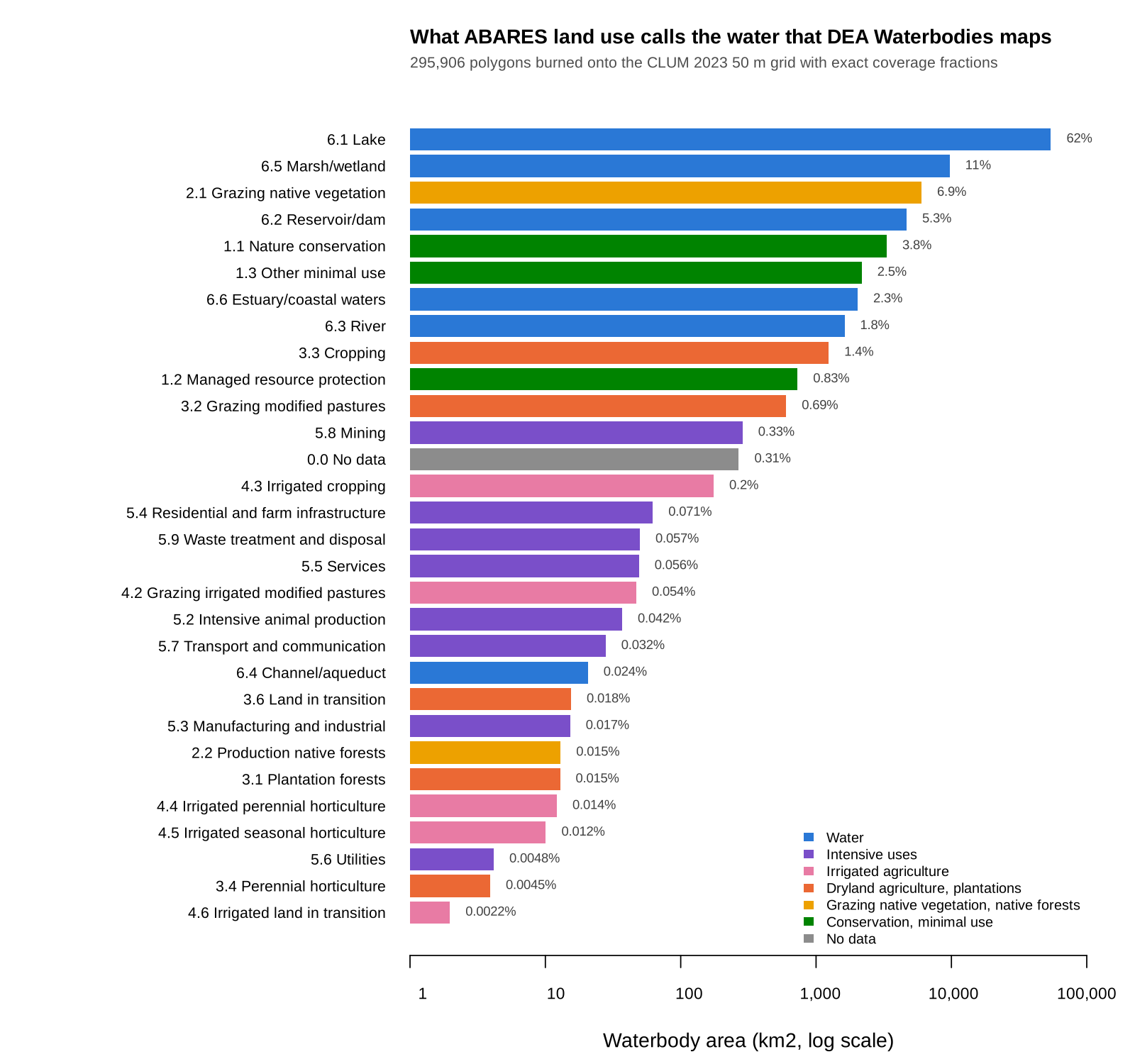
Grouped by ALUM secondary class, 82.7% of DEA waterbody area is water in CLUM: lakes 62%, marsh/wetland 11%, reservoir/dam 5.3%. The biggest non-water class is grazing native vegetation at 6.9%, then nature conservation at 3.8%.

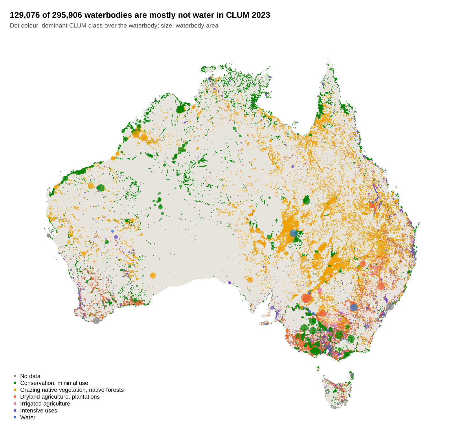
Waterbody area by CLUM land use class, log scale

By count, 129,076 of the 295,906 waterbodies are mostly not water in CLUM. They are small (median 1.1 ha), 13,080 km2 in total: mostly ephemeral water that CLUM labels by the land use around it.

Waterbodies that are mostly not water in CLUM, by dominant class