An Icechunk repository holds array data together with versioned, transactional metadata: which chunks exist, where their bytes live, and how the arrays have changed over time. tabularberg reads that metadata directly, so you can ask questions of a store as SQL tables before deciding which data to fetch.
This vignette uses a public store with no credentials: 44 years of NOAA OISST v2.1 daily sea surface temperature. Each chunk is a virtual reference to a byte range in one of NOAA’s netCDF files on AWS.
library(tabularberg)
library(DBI)

oisst <- "https://data.source.coop/ausantarctic/ausantarctic-scratch/oisst/oisst-v2.1-daily/icechunk"
con <- dbConnect(Icechunk(), oisst)
con
#> <IcechunkConnection> branch main @ 0MYSJ33RPR7A5VJJE040
dbListTables(con)
#>  [1] "meta"      "arrays"    "sources"   "branches"  "tags"      "ancestry"  "nodes"     "refs_anom"
#>  [9] "refs_err"  "refs_ice"  "refs_lat"  "refs_lon"  "refs_sst"  "refs_time" "refs_zlev"
What is in the store
arrays has one row per array, in the byterefs layout:
kind, dimensions, shape, chunking and data type.
dbGetQuery(con, 'SELECT "array", kind, dims, shape, chunks, dtype FROM arrays')
#>   array  kind                        dims              shape         chunks dtype
#> 1  anom  data ["time","zlev","lat","lon"] [16482,1,720,1440] [1,1,720,1440]   <i2
#> 2   err  data ["time","zlev","lat","lon"] [16482,1,720,1440] [1,1,720,1440]   <i2
#> 3   ice  data ["time","zlev","lat","lon"] [16482,1,720,1440] [1,1,720,1440]   <i2
#> 4   lat coord                     ["lat"]              [720]          [720]   <f8
#> 5   lon coord                     ["lon"]             [1440]         [1440]   <f8
#> 6   sst  data ["time","zlev","lat","lon"] [16482,1,720,1440] [1,1,720,1440]   <i2
#> 7  time coord                    ["time"]            [16482]        [16482]   <f8
#> 8  zlev coord                    ["zlev"]                [1]            [1]   <f8
nodes is Icechunk’s own view, and ancestry
the commit history of the branch.
dbGetQuery(con, "SELECT path, shape, num_chunks FROM nodes WHERE type = 'array'")
#>    path            shape  num_chunks
#> 1 /anom 16482,1,720,1440 16482,1,1,1
#> 2  /err 16482,1,720,1440 16482,1,1,1
#> 3  /ice 16482,1,720,1440 16482,1,1,1
#> 4  /lat              720           1
#> 5  /lon             1440           1
#> 6  /sst 16482,1,720,1440 16482,1,1,1
#> 7 /time            16482           1
#> 8 /zlev                1           1
dbGetQuery(con, "SELECT snapshot_id, written_at, message FROM ancestry")
#>            snapshot_id               written_at
#> 1 0MYSJ33RPR7A5VJJE040 2026-11-02T06:11:32.973Z
#> 2 1CECHNKREP0F1RSTCMT0 2026-11-02T06:11:32.662Z
#>                                                                 message
#> 1 mdim-refs flat store /v/work/oisst-v2.1-daily/out/flat, target public
#> 2                                                Repository initialized
Chunk references as rows
Each array also has a refs_<array> table with one
row per chunk. dim_0, dim_1, … are the chunk’s
indices, and path, offset and
size give the byte range it points to. sst is
chunked one day at a time, so dim_0 is the day number since
1981-09-01:
day <- as.integer(as.Date("2024-02-01") - as.Date("1981-09-01"))
dbGetQuery(con, sprintf('SELECT dim_0, path, "offset", size FROM refs_sst WHERE dim_0 = %d', day))
#>   dim_0
#> 1 15493
#>                                                                                                                                 path
#> 1 https://noaa-cdr-sea-surface-temp-optimum-interpolation-pds.s3.amazonaws.com/data/v2.1/avhrr/202402/oisst-avhrr-v02r01.20240201.nc
#>   offset   size
#> 1  47587 671857
That query reads only the chunk references it needs. When the
WHERE clause narrows dim_k with plain
comparisons, tabularberg fetches just that slab of chunks, and on stores
with split manifests only the manifests covering it. The SQL engine
still applies the full predicate, so results are the same as reading the
whole table. Joins are narrowed too. For example, does each day’s
ice chunk come from the same file as its sst
chunk?
dbGetQuery(con, "
  SELECT count(*) AS days, sum(s.path = i.path) AS same_file
  FROM refs_sst s JOIN refs_ice i ON s.dim_0 = i.dim_0
  WHERE s.dim_0 BETWEEN 15462 AND 15827")
#>   days same_file
#> 1  366       366
The filter on s.dim_0 carries across
s.dim_0 = i.dim_0, so both tables are read for that year
only.
Whole-table questions work as well, such as how much netCDF the
sst array references:
dbGetQuery(con, "SELECT count(*) AS chunks, sum(size) / 1e9 AS gigabytes FROM refs_sst")
#>   chunks gigabytes
#> 1  16482  11.03335
sources lists every referenced file. It reads every
array’s references, so later queries are answered from those cached
tables.
src <- dbReadTable(con, "sources")
nrow(src)
#> [1] 16482
basename(src$source[c(1, nrow(src))])
#> [1] "oisst-avhrr-v02r01.19810901.nc" "oisst-avhrr-v02r01.20261016.nc"
dbplyr
The connection works with dbplyr. Filters on dim_k are
pushed down in the same way.
library(dplyr, warn.conflicts = FALSE)
refs <- tbl(con, "refs_ice")
q <- refs |>
  filter(dim_0 >= 15462, dim_0 < 15462 + 366) |>
  summarise(chunks = n(), megabytes = sum(size, na.rm = TRUE) / 1e6)
show_query(q)
#> <SQL>
#> SELECT COUNT(*) AS `chunks`, SUM(`size`) / 1000000.0 AS `megabytes`
#> FROM `refs_ice`
#> WHERE (`dim_0` >= 15462.0) AND (`dim_0` < (15462.0 + 366.0))
collect(q)
#> # A tibble: 1 × 2
#>   chunks megabytes
#>    <int>     <dbl>
#> 1    366    20.995
dbDisconnect(con)
SQL runs on an in-memory SQLite copy by default. Use
dbConnect(Icechunk(), oisst, sql = "duckdb") for large
reference tables: they are then handed to DuckDB as Arrow record batches
built in Rust. In DuckDB offset and array are
reserved words, so quote them as above. ic_refs_arrow()
returns the same tables as an Arrow stream directly.
Time travel on a local catalogue
The public store is read-only and has a single commit. To see versioning at work, copy its references into a local repository. This copies only references: the chunks stay on NOAA’s bucket, and authorising that container lets the local repository read them.
noaa <- "https://noaa-cdr-sea-surface-temp-optimum-interpolation-pds.s3.amazonaws.com/"
pub <- ic_session_readonly(ic_repo_open(oisst), branch = "main")
local <- file.path(tempdir(), "oisst-catalogue")
repo <- ic_repo_from_byterefs(ic_to_byterefs(pub), local, authorize = noaa,
                              message = "copy of the public OISST references")
ic_tag_create(repo, "public", ic_branches(repo)$snapshot_id[1])
Next, add a curated array sst_2024 holding the 366 days
of 2024. Its rows are written in a transaction, which becomes one
Icechunk commit.
cg <- dbConnect(Icechunk(), local, authorize = noaa)
a <- dbReadTable(cg, "arrays")
y <- a[a$array == "sst", ]
y$array <- "sst_2024"
y$shape <- "[366,1,720,1440]"
d0 <- as.integer(as.Date("2024-01-01") - as.Date("1981-09-01"))
r <- dbGetQuery(cg, sprintf("SELECT * FROM refs_sst WHERE dim_0 BETWEEN %d AND %d", d0, d0 + 365))
r$dim_0 <- r$dim_0 - d0

dbBegin(cg)
dbAppendTable(cg, "arrays", y)
#> [1] 1
dbAppendTable(cg, "refs_sst_2024", r[c("dim_0", "dim_1", "dim_2", "dim_3", "path", "offset", "size")])
#> [1] 366
dbCommit(cg, "sst_2024: the days of 2024 as their own array")
dbGetQuery(cg, "SELECT snapshot_id, message FROM ancestry")
#>            snapshot_id                                       message
#> 1 SJ078RSTHBV96XGJ6S2G sst_2024: the days of 2024 as their own array
#> 2 M1W1NR8213ECB56VJTTG           copy of the public OISST references
#> 3 1CECHNKREP0F1RSTCMT0                        Repository initialized
The tag still sees the repository as it was before:
then <- dbConnect(Icechunk(), local, tag = "public", authorize = noaa)
"refs_sst_2024" %in% dbListTables(then)
#> [1] FALSE
"refs_sst_2024" %in% dbListTables(cg)
#> [1] TRUE
dbDisconnect(then); dbDisconnect(cg)
Connections can also pin a snapshot. Tag and snapshot
connections are read-only.
Decoding a slab
The tables say where the bytes are. To decode them, hand an Icechunk
session to pizzarr.
ic_pizzarr_store() wraps a session as a pizzarr store, so
pizzarr’s R code reads it. These chunks use netCDF-4’s shuffle and zlib
codecs, which pizzarr’s R decoder gains in the mdsumner/pizzarr fork
(branch icechunk-handoff). That fork also has
IcechunkStore, which reads through its Rust (zarrs)
backend.
s <- ic_session_readonly(ic_repo_open(local, authorize = noaa), branch = "main")
z <- pizzarr::zarr_open(ic_pizzarr_store(s), mode = "r", path = "sst_2024")
i <- 32L   # 2024-02-01
x <- z$get_item(list(pizzarr::slice(i, i), pizzarr::slice(1L, 1L),
                     pizzarr::slice(1L, 720L), pizzarr::slice(1L, 1440L)))$data
at <- z$get_attrs()$to_list()
sst <- x[1, 1, , ]
sst[sst == at[["_FillValue"]]] <- NA
sst <- sst * at$scale_factor
range(sst, na.rm = TRUE)
#> [1] -1.80 31.89

lon <- seq(0.125, 359.875, by = 0.25)
lat <- seq(-89.875, 89.875, by = 0.25)
pal <- hcl.colors(64, "Reds 3", rev = TRUE)
lim <- c(-2, 35)
layout(matrix(1:2, 1), widths = c(9, 1))
par(mar = c(3, 3, 2, 0.5), mgp = c(1.8, 0.5, 0), las = 1, cex.axis = 0.8)
plot(NA, xlim = c(0, 360), ylim = c(-90, 90), asp = 1, xaxs = "i", yaxs = "i",
     xlab = "longitude", ylab = "latitude",
     main = "Sea surface temperature, 2024-02-01 (OISST v2.1)", font.main = 1, cex.main = 0.95)
rect(0, -90, 360, 90, col = "grey80", border = NA)   # land and missing: grey
image(lon, lat, t(sst), col = pal, zlim = lim, useRaster = TRUE, add = TRUE)
par(mar = c(3, 0.5, 2, 3))
image(1, seq(lim[1], lim[2], length.out = 64), t(seq_len(64)), col = pal, axes = FALSE, xlab = "", ylab = "", useRaster = TRUE)
axis(4); mtext("°C", side = 3, line = 0.3, cex = 0.8)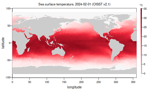
plot of chunk sst-2024-02-01
Only the one 2024-02-01 chunk was fetched: a single byte range from
oisst-avhrr-v02r01.20240201.nc.