Why topology?
wkpool represents geometry as segments referencing a shared vertex pool. Topology emerges naturally: shared edges, neighbours, and ring structure become simple lookups.
Simple features store geometry as complete coordinate sequences per feature. Two adjacent polygons duplicate their shared boundary, which wastes space and needs spatial predicates (GEOS) to rediscover adjacency.
Basic workflow
Create two adjacent squares sharing an edge:
library(wk)
library(wkpool)

# Two adjacent unit squares
poly1 <- wkt("POLYGON ((0 0, 1 0, 1 1, 0 1, 0 0))")
poly2 <- wkt("POLYGON ((1 0, 2 0, 2 1, 1 1, 1 0))")
geoms <- c(poly1, poly2)
Establish topology
pool <- establish_topology(geoms)
pool
#> <wkpool[8 segments, 10 vertices]>
#> [1] <segment: 1->2>  <segment: 2->3>  <segment: 3->4>  <segment: 4->5>
#> [5] <segment: 6->7>  <segment: 7->8>  <segment: 8->9>  <segment: 9->10>
At this stage, vertices are indexed but not yet merged: the shared edge exists as duplicate coordinate pairs.
Inspect the raw state
topology_report(pool)
#> $n_vertices_raw
#> [1] 10
#>
#> $n_vertices_unique
#> [1] 6
#>
#> $n_duplicate_vertices
#> [1] 4
#>
#> $n_near_miss_vertices
#> [1] 0
#>
#> $n_segments
#> [1] 8
#>
#> $n_shared_edges
#> [1] 1
#>
#> $n_features
#> [1] 2
Access the pool components
pool_vertices(pool)
#>    .vx x y
#> 1    1 0 0
#> 2    2 1 0
#> 3    3 1 1
#> 4    4 0 1
#> 5    5 0 0
#> 6    6 1 0
#> 7    7 2 0
#> 8    8 2 1
#> 9    9 1 1
#> 10  10 1 0
pool_segments(pool)
#>   .vx0 .vx1 .feature .path
#> 1    1    2        1     1
#> 2    2    3        1     1
#> 3    3    4        1     1
#> 4    4    5        1     1
#> 5    6    7        2     2
#> 6    7    8        2     2
#> 7    8    9        2     2
#> 8    9   10        2     2
pool_feature(pool)
#> [1] 1 1 1 1 2 2 2 2
Merge coincident vertices
pool <- merge_coincident(pool)
topology_report(pool)
#> $n_vertices_raw
#> [1] 6
#>
#> $n_vertices_unique
#> [1] 6
#>
#> $n_duplicate_vertices
#> [1] 0
#>
#> $n_near_miss_vertices
#> [1] 0
#>
#> $n_segments
#> [1] 8
#>
#> $n_shared_edges
#> [1] 1
#>
#> $n_features
#> [1] 2
After merging, shared edge vertices reference the same pool indices.
Adjacency discovery
Shared edges
find_shared_edges(pool)
#>   edge_key .vx0 .vx1 .feature segment_idx features
#> 2      2-3    2    3        1           2     1, 2
#> 8      2-3    2    3        2           8     1, 2
Returns segment indices that appear in multiple features.
Internal boundaries
For polygon data, shared edges with opposite winding indicate true internal boundaries (not self-shared rings):
find_internal_boundaries(pool)
#> <wkpool[2 segments, 6 vertices]>
#> [1] <segment: 2->3> <segment: 3->2>
Neighbour graph
find_neighbours(pool)
#>   feature_a feature_b
#> 3         1         2
Returns a data frame of feature pairs that share an edge.
Ring and cycle analysis
Topology enables ring discovery without parsing WKT structure.
Find closed cycles
cycles <- find_cycles(pool)
cycles
#> [[1]]
#> [1] 1 2 3 4
#>
#> [[2]]
#> [1] 2 5 6 3
#>
#> attr(,"path")
#> [1] 1 2
Classify by winding
Signed area distinguishes outer rings from holes. Following the SF convention, negative area indicates an outer ring, positive indicates a hole:
# Area of the first cycle
cycle_signed_area(cycles[[1]], pool_vertices(pool))
#> [1] 1

# Classify all cycles
classify_cycles(pool)
#>   cycle area  type .path .feature
#> 1     1    1 outer     1        1
#> 2     2    1 outer     2        2
Use reverse_cycle() to flip winding if needed.
Arc-node topology
Arcs are maximal sequences of segments passing through degree-2 vertices. Nodes are vertices where degree != 2 (branch points or endpoints).
vertex_degree(pool)
#> 1 2 3 4 5 6
#> 2 4 4 2 2 2
find_nodes(pool)
#> [1] 2 3
find_arcs(pool)
#> [[1]]
#> [1] 2 1 4 3
#>
#> [[2]]
#> [1] 2 3
#>
#> [[3]]
#> [1] 2 5 6 3
#>
#> [[4]]
#> [1] 2 3
arc_node_summary(pool)
#> $n_vertices
#> [1] 6
#>
#> $n_nodes
#> [1] 2
#>
#> $n_arcs
#> [1] 4
#>
#> $degree_distribution
#> deg
#> 2 4
#> 4 2
#>
#> $arc_length_distribution
#> arc_lengths
#> 1 3
#> 2 2
#>
#> $mean_arc_length
#> [1] 2
The two squares share an edge and each square carries its own copy of
it, so the shared vertices have degree 4 and the shared edge comes back
as two arcs, one per square. In the quotient graph a duplicated boundary
counts once: the shared edge is a single arc, and its end vertices stay
nodes because three distinct edges meet there. On a coverage with long
shared boundaries the difference is large (on silicate’s
inlandwaters, 5,418 arcs and 2,619 nodes by default, 201
arcs and 13 nodes in the quotient graph). Use
quotient = TRUE for polygon coverages.
find_nodes(pool, quotient = TRUE)
#> [1] 2 3
find_arcs(pool, quotient = TRUE)
#> [[1]]
#> [1] 2 1 4 3
#>
#> [[2]]
#> [1] 2 3
#>
#> [[3]]
#> [1] 2 5 6 3
Round-trip to WKT
Convert topology back to standard geometry formats:
# Arcs as linestrings
arcs_to_wkt(pool)
#> <wk_wkt[4]>
#> [1] LINESTRING (1 0, 0 0, 0 1, 1 1) LINESTRING (1 0, 1 1)
#> [3] LINESTRING (1 0, 2 0, 2 1, 1 1) LINESTRING (1 0, 1 1)

# Cycles as polygons
cycles_to_wkt(pool)
#> <wk_wkt[2]>
#> [1] POLYGON ((0 0, 1 0, 1 1, 0 1, 0 0)) POLYGON ((1 0, 2 0, 2 1, 1 1, 1 0))

# Raw segments
segments_to_wkt(pool, type = "linestring")[1:3]
#> <wk_wkt[3]>
#> [1] LINESTRING (0 0, 1 0) LINESTRING (1 0, 1 1) LINESTRING (1 1, 0 1)
Periodic x (antimeridian)
Longitude wraps. Two hemispheres that meet at -180 and 180 have two
copies of the seam, and plain merging keeps them apart. With
period_x = 360 the copies fuse and the seam becomes an
ordinary shared boundary (coordinates are not moved):
hemi <- wk::as_wkb(c(
  "POLYGON ((-180 -60, 0 -60, 0 60, -180 60, -180 -60))",
  "POLYGON ((0 -60, 180 -60, 180 60, 0 60, 0 -60))"
))
hp <- establish_topology(hemi)
nrow(find_shared_edges(merge_coincident(hp)))
#> [1] 2
nrow(find_shared_edges(merge_coincident(hp, period_x = 360)))
#> [1] 8
Triangulation
Triangles can share the same vertex pool.
pool_triangulate() (experimental) ear cuts each polygon and
returns a wkpool_tri, and as_pslg() with
pool_holes() gives the input for constrained Delaunay
engines such as RTriangle. See
vignette("triangulation", package = "wkpool").
tri <- pool_triangulate(pool)
plot(tri, asp = 1)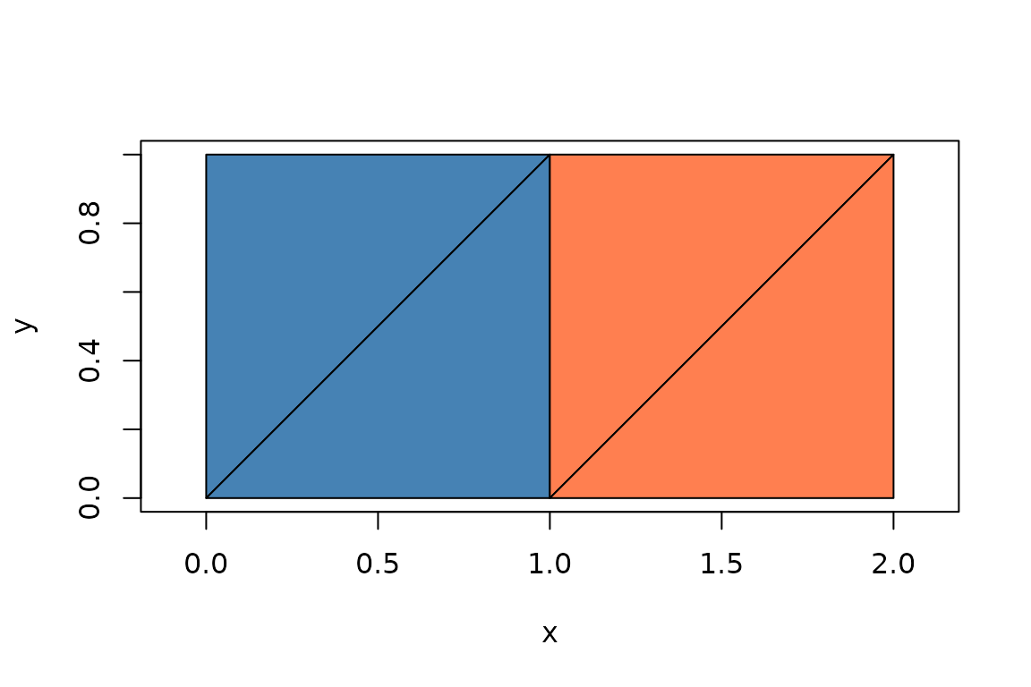
Subsetting and combining
Pools support [ subsetting; the full vertex pool is
retained:
pool[1:4]
#> <wkpool[4 segments, 6 vertices]>
#> [1] <segment: 1->2> <segment: 2->3> <segment: 3->4> <segment: 4->1>
Combine pools from different sources:
pool_a <- establish_topology(wk::wkt("POLYGON ((0 0, 1 0, 1 1, 0 1, 0 0))"))
pool_b <- establish_topology(wk::wkt("POLYGON ((5 5, 6 5, 6 6, 5 6, 5 5))"))
pool_combine(pool_a, pool_b)
#> <wkpool[8 segments, 10 vertices]>
#> [1] <segment: 1->2>  <segment: 2->3>  <segment: 3->4>  <segment: 4->5>
#> [5] <segment: 6->7>  <segment: 7->8>  <segment: 8->9>  <segment: 9->10>
Building a pool from tables
wkpool(vertices, segments) assembles a pool from a
vertex table and a segment table, the same shapes that
pool_vertices() and pool_segments() return.
This is the way in for data that is already indexed, such as a mesh read
from another format:
v <- data.frame(.vx = 1:4, x = c(0, 1, 1, 0), y = c(0, 0, 1, 1))
s <- data.frame(.vx0 = 1:4, .vx1 = c(2:4, 1L), .feature = 1L)
wkpool(v, s)
#> <wkpool[4 segments, 4 vertices]>
#> [1] <segment: 1->2> <segment: 2->3> <segment: 3->4> <segment: 4->1>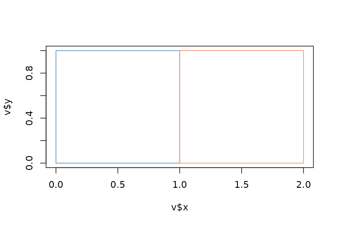
Related Work
Core topology/vertex-pool (hypertidy ecosystem)
| Package | Where | Relationship to wkpool |
|---|---|---|
| silicate | CRAN | Topological models: SC (edge-vertex), ARC
(shared boundaries), PATH, TRI. Its
silicate2 branch routes geometry through wkpool |
| unjoin | CRAN | Vertex deduplication via data frame normalization, used internally by silicate |
| wk | CRAN | Path/geometry indexing via wk_coords()
|
Mesh/triangulation
| Package | Where | Notes |
|---|---|---|
| decido | CRAN | Ear cutting, the engine for pool_triangulate()
(experimental) |
| RTriangle | CRAN | Shewchuk’s Triangle, constrained Delaunay with quality refinement;
takes as_pslg() and pool_holes()
|
| laridae | GitHub | Constrained Delaunay and meshing with CGAL |
| meshcore | GitHub | Mesh tables and tri_mesh() over further constrained
Delaunay engines |
| sfdct | CRAN | RTriangle wrapper for sf objects |
Adjacency (computed, not stored)
| Package | Where | Approach |
|---|---|---|
| sfdep | CRAN |
st_contiguity() computes on-demand |
| sf | CRAN |
st_touches(), st_relate() via GEOS,
recomputed each time |
Key distinction: wkpool differs from sf/spdep by
storing topology (shared edges are explicit) rather than
computing it on demand via GEOS. It is the lightweight,
wk-native machinery under silicate’s approach.