8913 days of five variables, one VRT, built from a catalogue
The GHRSST Multi-scale Ultra-high Resolution (MUR) sea surface temperature analysis is a daily global grid at 0.01 degrees (17999 x 36000 cells) from 2002-06-01. A cloud-optimised copy is published on source.coop as five Cloud Optimized GeoTIFFs per day, one per variable, with a STAC catalogue in stac-geoparquet form. The pipeline that produces it is AustralianAntarcticDivision/ghrsst-cogger.
This page builds one multidimensional VRT over the whole collection from the catalogue alone, then uses it for a regional map, a 24-year pixel series, the start of the anomaly record, and a sea ice snapshot.
Each item is one day; each asset is one COG. Not every variable covers the whole record:
import pandas as pdcoverage = []for key in rows[-1]["assets"]: days = [r["datetime"] for r in rows if r["assets"].get(key)] band = rows[-1]["assets"][key]["raster:bands"][0] coverage.append({"asset": key, "days": len(days),"first": f"{days[0]:%Y-%m-%d}", "last": f"{days[-1]:%Y-%m-%d}","dtype": band.get("data_type"), "scale": band.get("scale"),"offset": band.get("offset"), "unit": band.get("unit")})pd.DataFrame(coverage)
No COG was opened: the grid, CRS, dates and each variable’s storage came from the catalogue. Days without a file for a variable are left empty and read as nodata. The VRT is plain XML; its head:
lines = vrt_path.read_text().splitlines()print("\n".join(l[:110] for l in lines[:28]))
from osgeo import gdalgdal.UseExceptions()ds = gdal.OpenEx(str(vrt_path), gdal.OF_MULTIDIM_RASTER)root = ds.GetRootGroup()for name in root.GetMDArrayNames(): a = root.OpenMDArray(name) shape = [d.GetSize() for d in a.GetDimensions()]print(f"{name:17s}{shape} unit={a.GetUnit()!r}")
time              [8913]  unit='days since 1970-01-01'
y                 [17999]  unit=''
x                 [36000]  unit=''
analysed_sst      [8913, 17999, 36000]  unit='kelvin'
analysis_error    [8913, 17999, 36000]  unit='kelvin'
mask              [8913, 17999, 36000]  unit=''
sea_ice_fraction  [8913, 17999, 36000]  unit='fraction (between 0 and 1)'
sst_anomaly       [8913, 17999, 36000]  unit='kelvin'
The grid and dates come back as coordinate arrays. A few helpers turn longitude, latitude and dates into array indices, and temperatures into degrees Celsius. The unit is whatever the catalogue records, read here rather than assumed; only absolute temperatures are shifted from kelvin, not differences such as the anomaly or the error estimate.
import numpy as nptimes = np.datetime64("1970-01-01") + root.OpenMDArray("time").ReadAsArray().astype("int64").astype("timedelta64[D]")def col(lon): returnint(round((lon +179.995) /0.01))def row(lat): returnint(round((89.995- lat) /0.01))def day(date): returnint(np.where(times == np.datetime64(date))[0][0])def celsius(values, unit, absolute=True): kelvin = unit.lower() in ("kelvin", "k")return values -273.15if (kelvin and absolute) else valuessst = root.OpenMDArray("analysed_sst")print(times[[0, -1]], sst.GetUnit())
['2002-06-01' '2026-10-25'] kelvin
A regional map for one day
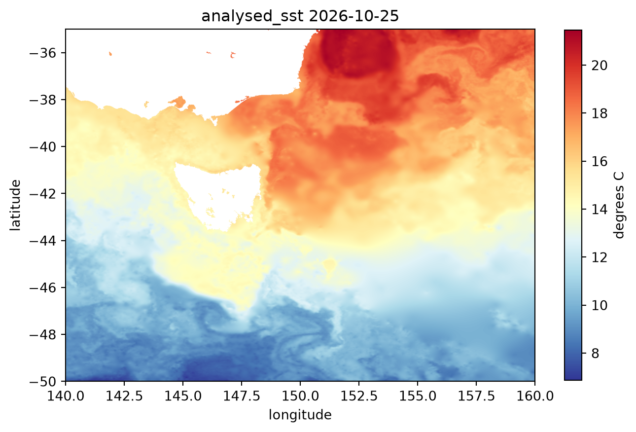
The Tasman Sea and Southern Ocean around Tasmania on the most recent day: one window of one COG.
Analysed SST, 140-160E 35-50S, most recent day in the catalogue.
One pixel through 24 years
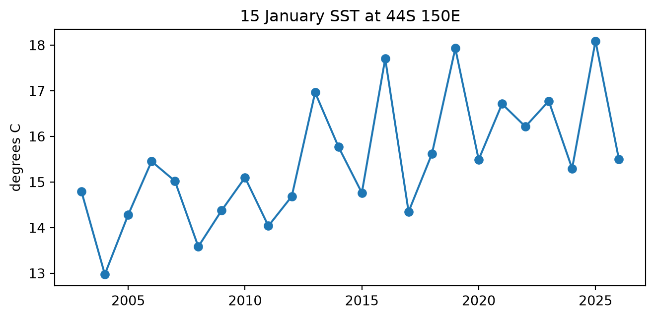
Mid-January at 44S 150E, east of Tasmania, for every January in the record. Each value comes from a different COG, and only those 24 files are opened: the time is spent on one remote request per day, not on the size of the collection.
def read_point(var, t, y, x): a = root.OpenMDArray(var) v = a.GetUnscaled().ReadAsArray(array_start_idx=[t, y, x], count=[1, 1, 1]).item()return celsius(v, a.GetUnit(), absolute=(var =="analysed_sst"))januaries = [i for i, d inenumerate(times) ifstr(d).endswith("-01-15")]t0 = time.time()series = [read_point("analysed_sst", i, row(-44), col(150)) for i in januaries]print(f"{len(series)} days in {time.time() - t0:.1f} s")years = [int(str(times[i])[:4]) for i in januaries]fig, ax = plt.subplots(figsize=(8, 3.5))ax.plot(years, series, marker="o")ax.set_ylabel("degrees C"); ax.set_title("15 January SST at 44S 150E")plt.show()
24 days in 69.0 s
Analysed SST on 15 January each year at 44S 150E.
Note
A strided read (array_step=[365, 1, 1]) would be the natural way to ask for one day per year, but in GDAL 3.13 a stride that crosses from one source to the next fails with arrayStartIdx[0] = ... >= 1; stepping within a single source works. Reading the chosen days individually, as above, avoids it.
Where a variable starts
sst_anomaly exists only from 2014-01-01. In the VRT it is one array over the whole record; days before its first file are nodata:
dates = ["2013-12-30", "2013-12-31", "2014-01-01", "2014-01-02", "2014-01-03"]sst_vals = [read_point("analysed_sst", day(d), row(-44), col(150)) for d in dates]anom_vals = [read_point("sst_anomaly", day(d), row(-44), col(150)) for d in dates]pd.DataFrame({"date": dates, "analysed_sst": np.round(sst_vals, 3),"sst_anomaly": np.round(anom_vals, 3)})
date
analysed_sst
sst_anomaly
0
2013-12-30
14.163
NaN
1
2013-12-31
14.063
NaN
2
2014-01-01
14.141
-0.264
3
2014-01-02
14.483
0.085
4
2014-01-03
14.550
0.079
Sea ice off East Antarctica
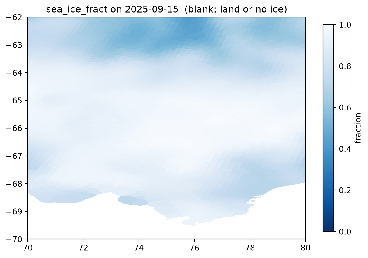
sea_ice_fraction off Prydz Bay (62-70S, 70-80E) on 15 September 2025, near the winter maximum:
Any reader of GDAL’s multidimensional API can use the VRT. With an xarray backend for GDAL the five arrays become one lazy Dataset; selections are read on demand.
import xarray as xrcube = xr.open_dataset(vrt_path, engine="gdalxarray")cube
<xarray.Dataset> Size: 208TB
Dimensions:           (time: 8913, y: 17999, x: 36000)
Coordinates:
  * time              (time) datetime64[ns] 71kB 2002-06-01 ... 2026-10-25
  * y                 (y) float64 144kB 89.99 89.98 89.97 ... -89.98 -89.99
  * x                 (x) float64 288kB -180.0 -180.0 -180.0 ... 180.0 180.0
  * crs               int64 8B 0
Data variables:
    analysed_sst      (time, y, x) float64 46TB ...
    analysis_error    (time, y, x) float64 46TB ...
    mask              (time, y, x) float32 23TB ...
    sea_ice_fraction  (time, y, x) float64 46TB ...
    sst_anomaly       (time, y, x) float64 46TB ...
Indexes:
    crs      CRSIndex (crs=EPSG:4326)
GEOGCRS["WGS 84",ENSEMBLE["World Geodetic System 1984 ensemble",MEMBER["World Geodetic System 1984 (Transit)"],MEMBER["World Geodetic System 1984 (G730)"],MEMBER["World Geodetic System 1984 (G873)"],MEMBER["World Geodetic System 1984 (G1150)"],MEMBER["World Geodetic System 1984 (G1674)"],MEMBER["World Geodetic System 1984 (G1762)"],MEMBER["World Geodetic System 1984 (G2139)"],MEMBER["World Geodetic System 1984 (G2296)"],ELLIPSOID["WGS 84",6378137,298.257223563,LENGTHUNIT["metre",1]],ENSEMBLEACCURACY[2.0]],PRIMEM["Greenwich",0,ANGLEUNIT["degree",0.0174532925199433]],CS[ellipsoidal,2],AXIS["geodetic latitude (Lat)",north,ORDER[1],ANGLEUNIT["degree",0.0174532925199433]],AXIS["geodetic longitude (Lon)",east,ORDER[2],ANGLEUNIT["degree",0.0174532925199433]],USAGE[SCOPE["Horizontal component of 3D system."],AREA["World."],BBOX[-90,-180,90,180]],ID["EPSG",4326]]
array(0)
analysed_sst
(time, y, x)
float64
...
units :
kelvin
grid_mapping :
crs
[5775303132000 values with dtype=float64]
analysis_error
(time, y, x)
float64
...
units :
kelvin
grid_mapping :
crs
[5775303132000 values with dtype=float64]
mask
(time, y, x)
float32
...
grid_mapping :
crs
[5775303132000 values with dtype=float32]
sea_ice_fraction
(time, y, x)
float64
...
units :
fraction (between 0 and 1)
grid_mapping :
crs
[5775303132000 values with dtype=float64]
sst_anomaly
(time, y, x)
float64
...
units :
kelvin
grid_mapping :
crs
[5775303132000 values with dtype=float64]
crs
CRSIndex (crs=EPSG:4326)
CRSIndex
<Geographic 2D CRS: EPSG:4326>
Name: WGS 84
Axis Info [ellipsoidal]:
- Lat[north]: Geodetic latitude (degree)
- Lon[east]: Geodetic longitude (degree)
Area of Use:
- name: World.
- bounds: (-180.0, -90.0, 180.0, 90.0)
Datum: World Geodetic System 1984 ensemble
- Ellipsoid: WGS 84
- Prime Meridian: Greenwich
v = cube.analysed_sst.sel(time="2025-02-14").sel(y=-44, x=150, method="nearest").load()float(celsius(v.values, cube.analysed_sst.attrs.get("units", "")))
18.281999999999982
Keeping it current
The VRT is a function of the catalogue, so rebuilding it whenever the catalogue changes keeps it current: here that takes a few seconds for the whole record, and it can be published next to the catalogue it was built from.