Curvilinear grids

Swaths and ocean model grids placed by 2D longitude and latitude, and warped by geolocation arrays.

Satellite swaths, ocean and atmosphere models on rotated or stretched grids: the cells are a regular array in index space, and each cell’s place on the earth is given by 2D longitude and latitude arrays. An affine geotransform cannot describe them.

A model grid in index space

The ROMS-style fixture stores temp on (s_rho, eta_rho, xi_rho), with lon_rho and lat_rho as 2D coordinates. gdalxarray keeps those as coordinates, so xarray’s plotting can place each cell:

roms = xr.open_dataset(fixture("index/roms-fan.zarr"), engine="gdalxarray")
roms["temp"].coords
Coordinates:
  * s_rho    (s_rho) float64 64B -0.9375 -0.8125 -0.6875 ... -0.1875 -0.0625
  * eta_rho  (eta_rho) int64 368B 0 1 2 3 4 5 6 7 8 ... 38 39 40 41 42 43 44 45
  * xi_rho   (xi_rho) int64 192B 0 1 2 3 4 5 6 7 8 ... 16 17 18 19 20 21 22 23
    lon_rho  (eta_rho, xi_rho) float64 9kB ...
    lat_rho  (eta_rho, xi_rho) float64 9kB ...
surf = roms["temp"].isel(s_rho=-1).where(roms["mask_rho"] > 0)
fig, axs = plt.subplots(1, 2, figsize=(11, 4.5), layout="constrained")
surf.plot(ax=axs[0], cmap="RdYlBu_r", add_colorbar=False)
axs[0].set_title("index space")
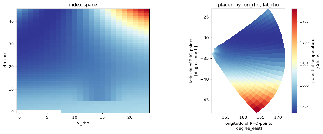
surf.plot(ax=axs[1], x="lon_rho", y="lat_rho", cmap="RdYlBu_r")
axs[1].set_title("placed by lon_rho, lat_rho"); axs[1].set_aspect(1 / np.cos(np.radians(-33)))
plt.show()

The same surface temperature by index (left) and placed by lon_rho/lat_rho (right): the grid fans out from the coast.

The vertical axis is index space too: depths come from the stretching parameters stored beside the data (Vtransform, Cs_r, hc, h, zeta), which gdalxarray reads as ordinary variables.

{k: float(roms[k]) for k in ["Vtransform", "Vstretching", "theta_s", "theta_b", "hc"]}
{'Vtransform': 2.0,
 'Vstretching': 4.0,
 'theta_s': 6.5,
 'theta_b': 1.5,
 'hc': 200.0}

A rotated-pole grid

A EURO-CORDEX-style window: regular in rotated longitude and latitude, with the true lon, lat as 2D coordinates and the rotation recorded in a CF grid_mapping variable.

rot = xr.open_dataset(fixture("index/rotated.zarr"), engine="gdalxarray")
rot["tas"].attrs, rot["rotated_pole"].attrs
({'grid_mapping': 'rotated_pole',
  'standard_name': 'air_temperature',
  'units': 'K'},
 {'grid_mapping_name': 'rotated_latitude_longitude',
  'grid_north_pole_latitude': 39.25,
  'grid_north_pole_longitude': -162.0})
fig, axs = plt.subplots(1, 2, figsize=(11, 4.2), layout="constrained")
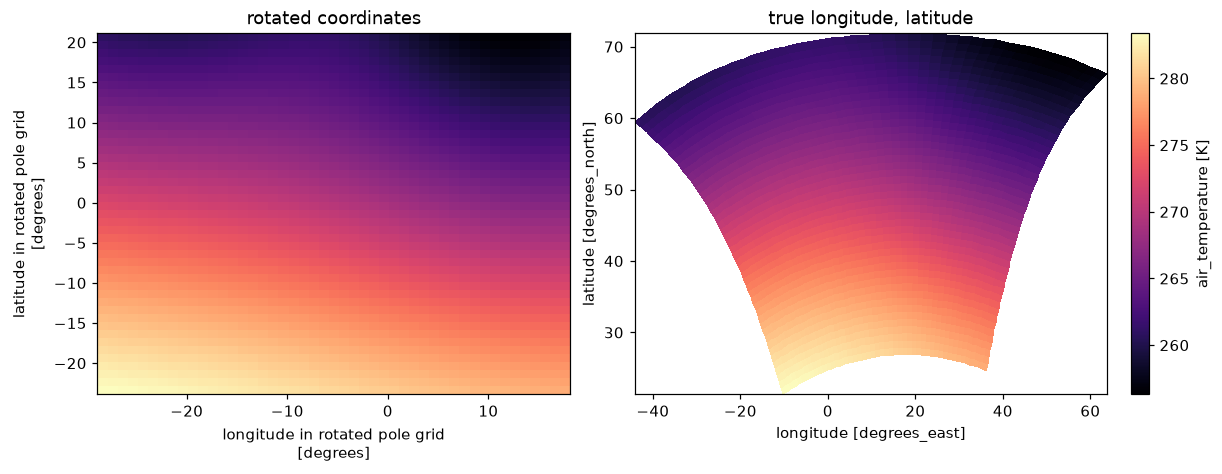
rot["tas"].plot(ax=axs[0], cmap="magma", add_colorbar=False)
axs[0].set_title("rotated coordinates")
rot["tas"].plot(ax=axs[1], x="lon", y="lat", cmap="magma")
axs[1].set_title("true longitude, latitude")
plt.show()

Near-surface temperature on the rotated grid: a rectangle in rotated coordinates, curved on the earth.

Warping by geolocation arrays

To regrid a curvilinear field, GDAL’s warper can use the 2D longitude and latitude directly (“geolocation arrays”). The recipe is a VRT with a GEOLOCATION metadata domain naming the arrays; gdalxarray.warp then forwards geoloc=True to gdal.WarpOptions.

The swath fixture is 120 x 160 cells with its longitudes and latitudes as two bands of a separate file:
swath = fixture("curvilinear/swath-120x160.tif")
lonlat = fixture("curvilinear/swath-120x160-lonlat.tif")

wgs84 = osr.SpatialReference(); wgs84.ImportFromEPSG(4326)
gdal.Translate("/vsimem/swath.vrt", swath, format="VRT")
v = gdal.Open("/vsimem/swath.vrt", gdal.GA_Update)
v.SetMetadata({"X_DATASET": lonlat, "X_BAND": "1", "Y_DATASET": lonlat, "Y_BAND": "2",
               "PIXEL_OFFSET": "0", "LINE_OFFSET": "0", "PIXEL_STEP": "1", "LINE_STEP": "1",
               "SRS": wgs84.ExportToWkt(), "GEOREFERENCING_CONVENTION": "PIXEL_CENTER"},
              "GEOLOCATION")
v = None

The fixture manifest gives target grids; one in Antarctic Polar Stereographic:

man = fixture_json("curvilinear/manifest.json")
case = next(c for c in man["cases"] if c["name"] == "swath-to-3031")
gt, W, H = case["geotransform"], case["width"], case["height"]
bbox = (gt[0], gt[3] + gt[5] * H, gt[0] + gt[1] * W, gt[3])

ll = xr.open_dataset(lonlat, engine="gdalxarray", multidim=False)["band_data"]
raw = xr.open_dataset(swath, engine="gdalxarray", multidim=False)["band_data"].isel(band=0)
warped = {m: xr.open_dataset(gdalxarray.warp("/vsimem/swath.vrt", crs=case["crs"], bbox=bbox,
                                             shape=(W, H), resampling=m, geoloc=True,
                                             nodata=-9999,
                                             errorThreshold=man["error_threshold"]),
                             engine="gdalxarray", multidim=False)["band_data"].isel(band=0)
          for m in ["near", "bilinear"]}
fig, axs = plt.subplots(1, 3, figsize=(13, 4), layout="constrained")
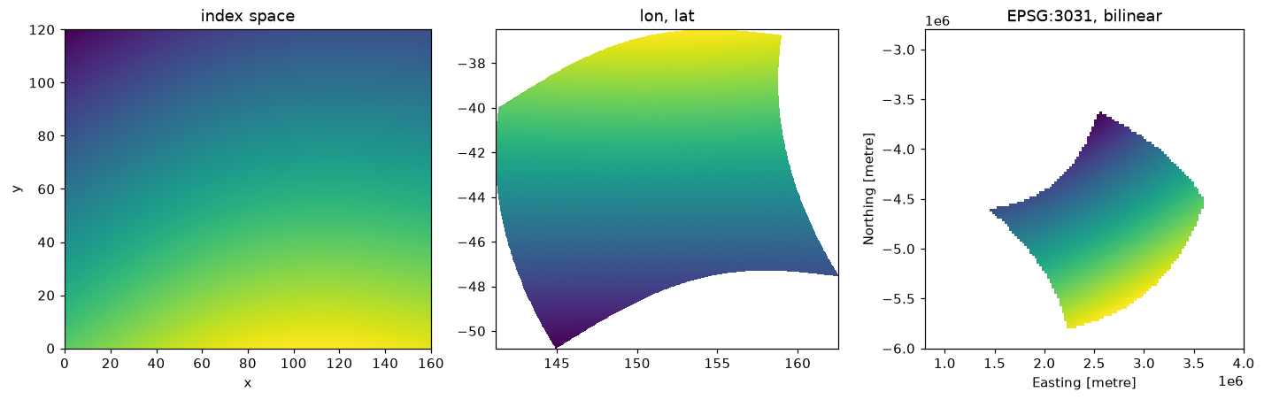
raw.plot(ax=axs[0], cmap="viridis", add_colorbar=False); axs[0].set_title("index space")
axs[1].pcolormesh(ll.isel(band=0), ll.isel(band=1), raw, cmap="viridis", shading="nearest")
axs[1].set_title("lon, lat"); axs[1].set_aspect(1 / np.cos(np.radians(-44)))
warped["bilinear"].plot(ax=axs[2], cmap="viridis", add_colorbar=False)
axs[2].set_aspect("equal"); axs[2].set_title("EPSG:3031, bilinear")
plt.show()

The swath in index space, its own longitude/latitude, and warped to EPSG:3031 by its geolocation arrays.

As on the Warping page, gdalxarray must match GDAL’s own read of the same recipe exactly; the fixture’s pinned oracle is reported:

rows = []
for r in case["results"]:
    if r["resampling"] not in warped:
        continue
    vrt = gdalxarray.warp("/vsimem/swath.vrt", crs=case["crs"], bbox=bbox, shape=(W, H),
                          resampling=r["resampling"], geoloc=True,
                          errorThreshold=man["error_threshold"])
    gx = xr.open_dataset(vrt, engine="gdalxarray", multidim=False,
                         mask_and_scale=False)["band_data"].values[0]
    ref = gdal.Open(vrt).ReadAsArray()
    pin = fixture_array("curvilinear/" + r["file"], "float32").reshape(H, W)
    eq = lambda a, b: float(np.mean((a == b) | (np.isnan(a) & np.isnan(b))))
    rows.append((r["resampling"], eq(gx, ref), eq(ref, pin)))
    assert np.array_equal(gx, ref, equal_nan=True)

import pandas as pd
pd.DataFrame(rows, columns=["resampling", "gdalxarray = GDAL VRT", "GDAL VRT = pinned"]) \
    .style.format("{:.2%}", subset=["gdalxarray = GDAL VRT", "GDAL VRT = pinned"]).hide(axis="index")
resampling gdalxarray = GDAL VRT GDAL VRT = pinned
near 100.00% 100.00%
bilinear 100.00% 76.09%

Rendered with GDAL 3.13.3, xarray 2026.4.1.dev32+g71cfb13ac, numpy 2.5.4, gdalxarray 0.5.1, rasterix 0.2.4.