tissot - Tissot Indicatrix for Map Projection Distortion • tissot

The Tissot Indicatrix characterizes local distortion in map projections. This package computes and plots indicatrixes using the PROJ library directly via the PROJ R package.

Derived (with permission) from Bill Huber’s GIS StackExchange answer.

Installation

# install.packages("pak")
pak::pak("tissot")

Quick start

tissot() returns a tibble of distortion properties. The second argument is the projection target; source defaults to EPSG:4326:

library(tissot)
tissot(c(147, -42), "+proj=utm +zone=55 +south")
#> Tissot indicatrix: 1 point, +proj=utm +zone=55 +south
#> # A tibble: 1 × 14
#>       x     y dx_dlam dy_dlam    dx_dphi dy_dphi
#>   <dbl> <dbl>   <dbl>   <dbl>      <dbl>   <dbl>
#> 1   147   -42 0.74396       0 6.1410e-16 0.99739
#> # ℹ 8 more variables: scale_h <dbl>, scale_k <dbl>,
#> #   scale_omega <dbl>, scale_a <dbl>, scale_b <dbl>,
#> #   scale_area <dbl>, angle_deformation <dbl>,
#> #   convergence <dbl>

Columns include: scale_h (meridional), scale_k (parallel), scale_a / scale_b (max/min singular values), scale_area, angle_deformation, and convergence.

Plotting indicatrixes

indicatrix() builds plottable ellipses. The dashed circle is the undistorted reference; the filled ellipse shows the projection’s distortion.

xy <- expand.grid(x = seq(0, 1e6, length.out = 5), y = seq(4900000, 5700000, length.out = 4))
lonlat <- tissot_unproject(xy, source = "+proj=utm +zone=55 +south")
tis <- tissot(lonlat, "+proj=utm +zone=55 +south")
plot(indicatrix(tis), scale = 3e4)
tissot_map()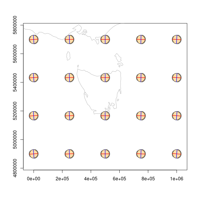

Tissot indicatrixes on a 5x4 grid across UTM zone 55S, showing near-circular ellipses confirming low distortion near the central meridian at 147°E, with slight elongation toward the zone edges

plot of chunk utm55

What does that top left indicatrix look like?

plot(indicatrix(tis)[1])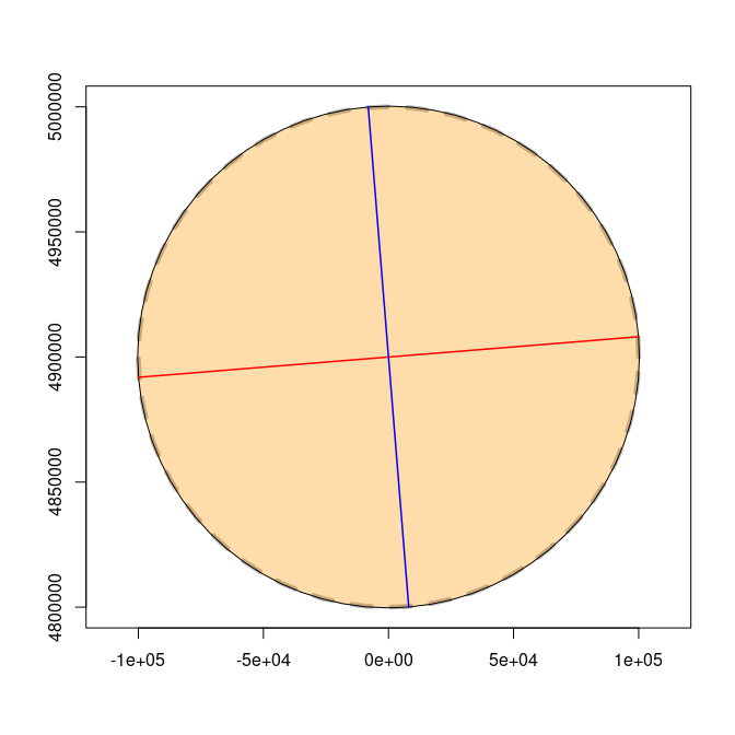

Single Tissot indicatrix from the top-left corner of the UTM zone 55S grid, showing a slightly tilted ellipse due to convergence away from the central meridian

plot of chunk topleft

Far from our UTM zone we are in a lot more trouble.

## UTM zone 55 is at 147 longitude (55 * 6 - 183)
tis <- tissot(cbind(100, -42), "+proj=utm +zone=55 +south")
plot(indicatrix(tis))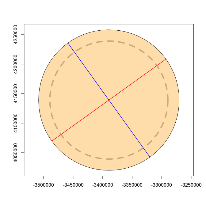

Single Tissot indicatrix for UTM zone 55S evaluated at longitude 100°E, far from the central meridian, showing extreme angular and areal distortion

plot of chunk very-bad-trouble


##  In Mercator we have well known problems 
tis <- tissot(cbind(147, -42), "+proj=merc")
plot(indicatrix(tis))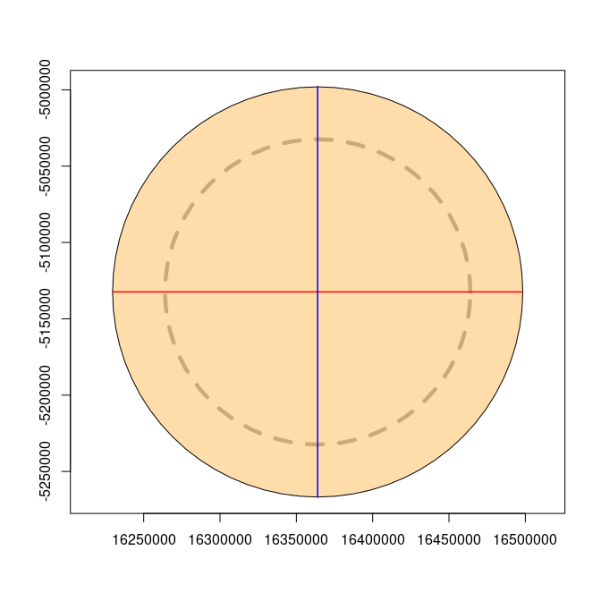

Tissot indicatrix for Mercator at latitude -42°, showing strong north-south stretching relative to east-west scale

plot of chunk very-bad-trouble


## close to the equator Mercator is ok (in exactly the same way that UTM Zone 55 is ok near 147E longitude)
tis <- tissot(cbind(147, 0), "+proj=merc")
plot(indicatrix(tis))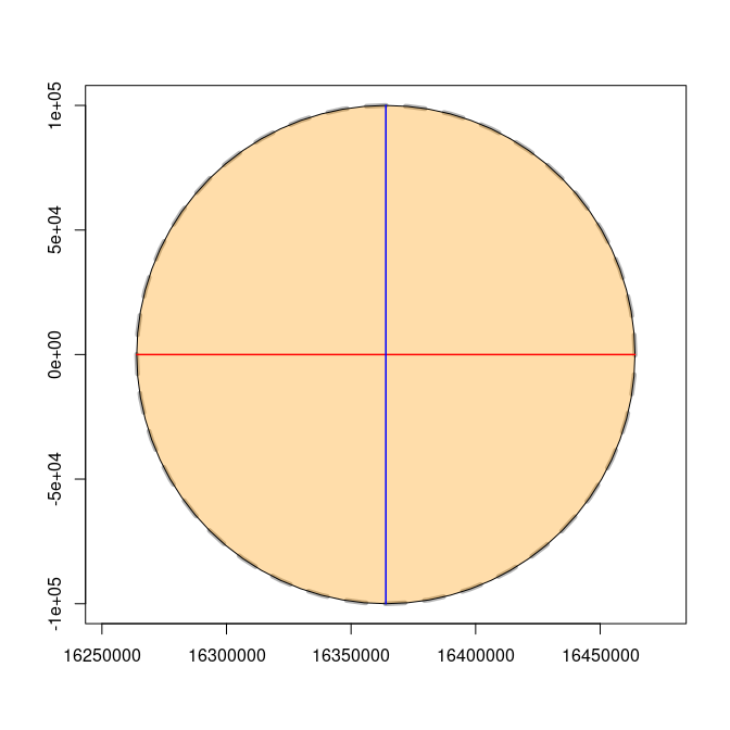

Tissot indicatrix for Mercator near the equator, showing a near-circular ellipse confirming low distortion close to latitude 0°

plot of chunk very-bad-trouble

Map projection is arbitrary.

xy <- expand.grid(seq(-150, 150, by = 30), seq(-60, 60, by = 30))
r <- tissot(xy, "+proj=robin")
ii <- indicatrix(r)
plot(ii, scale = 6e5, add = FALSE, show.axes  = TRUE, show.circle = TRUE)
tissot_map()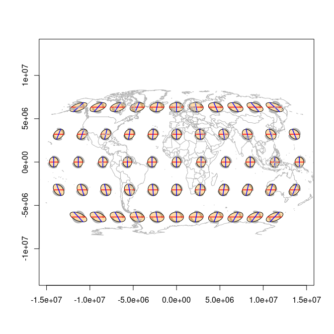

Grid of Tissot indicatrixes across the Robinson projection with world coastline overlay, showing rounder ellipses near the equator and increasing distortion toward the poles and edges

plot of chunk robinson

Distortion summary

summary(r)
#> Tissot indicatrix: 55 points
#>   Source CRS: EPSG:4326
#>   Target CRS: +proj=robin
#>   Areal scale:  min=0.8154  max=1.2004  mean=1.0095
#>   Angular def:  min=1.9369  max=51.8469  mean=21.3801 deg
#>   Scale h:      min=0.8856  max=1.3030  (meridional)
#>   Scale k:      min=0.8487  max=1.3555  (parallel)

Colour-coded distortion

Pass fill.by to colour ellipses by a distortion metric:

plot(ii, scale = 6e5, add = FALSE, fill.by = "scale_area")
tissot_map()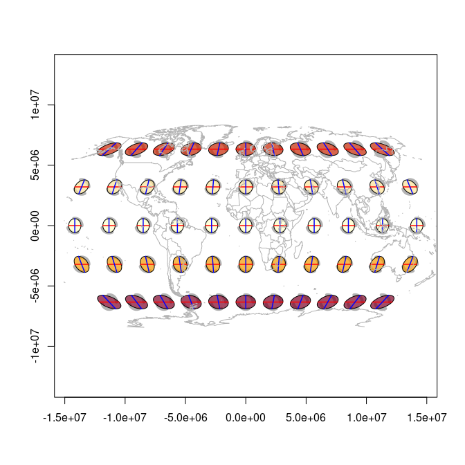

Tissot indicatrixes for the Robinson projection coloured by areal scale factor, with warm colours toward the poles indicating areas where the projection expands area

plot of chunk coloured

plot(ii, scale = 6e5, add = FALSE, fill.by = "angle_deformation")
tissot_map()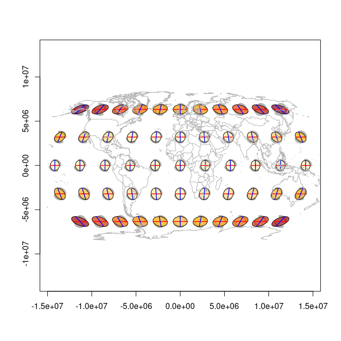

Tissot indicatrixes for the Robinson projection coloured by angular deformation in degrees, with warm colours in the corners showing where the projection distorts angles most

plot of chunk angle_deformation

Projection comparison

m <- tissot(xy, "+proj=moll")
plot(indicatrix(m), scale = 5e5, add = FALSE)
tissot_map()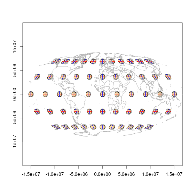

Grid of Tissot indicatrixes for the Mollweide equal-area projection, showing ellipses of consistent area but varying shape across the map

plot of chunk mollweide

merc_xy <- expand.grid(seq(-150, 150, by = 30), seq(-75, 75, by = 15))
me <- tissot(merc_xy, "+proj=merc")
plot(indicatrix(me), scale = 5e5, add = FALSE)
tissot_map()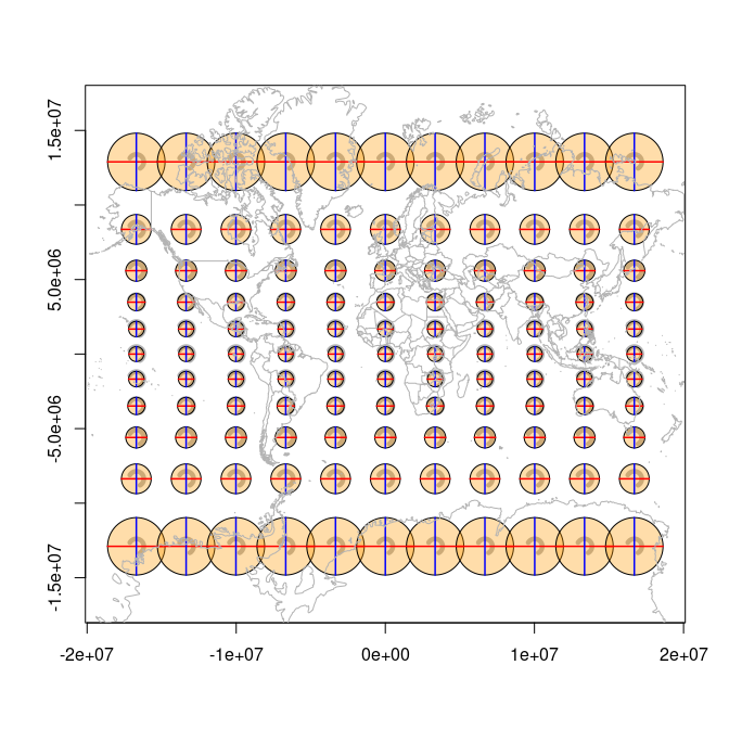

Grid of Tissot indicatrixes for the Mercator projection, showing circular ellipses near the equator that grow dramatically larger toward the poles while retaining their circular shape

plot of chunk mercator

Rich single-indicatrix plots

A single indicatrix with axes and reference circle:

ii2 <- indicatrix(c(147, -42), "+proj=lcc +lat_1=-36 +lat_2=-38 +lat_0=-37 +lon_0=145")
plot(ii2[[1]], scale = 1e4, add = FALSE, show.axes = TRUE, show.circle = TRUE)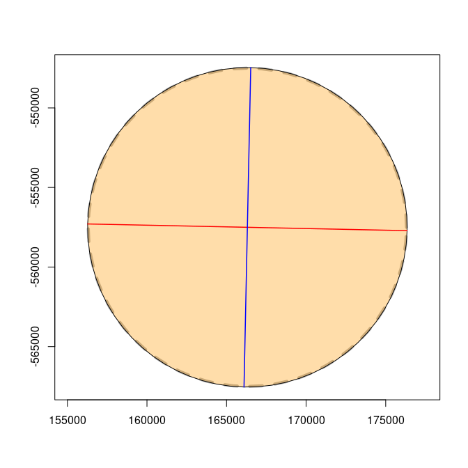

Single Tissot indicatrix for a Lambert Conformal Conic with standard parallels at -36 and -38 degrees, evaluated at 147°E 42°S, showing a near-circular ellipse indicating low distortion close to the standard parallels

plot of chunk single2

ii3 <- indicatrix(c(147, -42), "+proj=lcc +lat_1=-15 +lat_2=5 +lat_0=0 +lon_0=145")
plot(ii3[[1]], scale = 1e4, add = FALSE, show.axes = TRUE, show.circle = TRUE)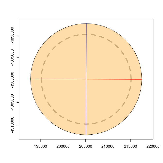

Single Tissot indicatrix for a Lambert Conformal Conic with standard parallels at -15 and +5 degrees, evaluated at 147°E 42°S, showing significant distortion far from the standard parallels

plot of chunk single3

Arbitrary projections

Lambert Conformal Conic

pxy <- expand.grid(seq(100, 200, by = 25), seq(-75, -45, by = 10))
p <- tissot(pxy, "+proj=lcc +lat_0=-60 +lon_0=147 +lat_1=-70 +lat_2=-55")
plot(indicatrix(p), scale = 3e5, add = FALSE, fill.by = "scale_area")
tissot_map()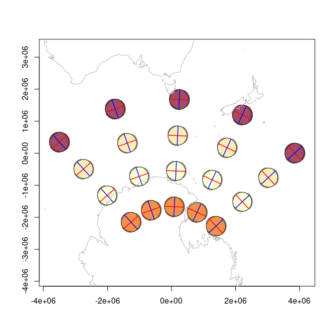

plot of chunk lcc

Universal Transverse Mercator

qxy <- expand.grid(seq(100, 200, by = 25), seq(-75, -45, by = 10))
p <- tissot(qxy, "EPSG:32755")
plot(indicatrix(p), scale = 3e5, add = FALSE, fill.by = "scale_area")
tissot_map()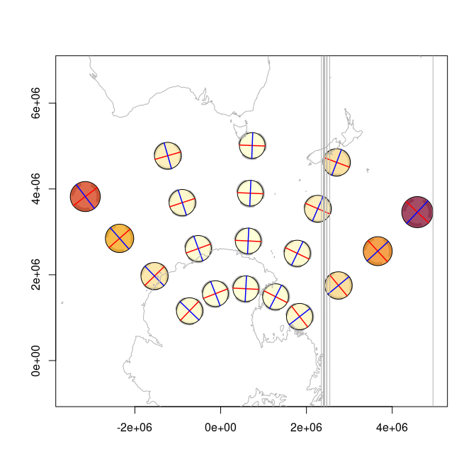

Tissot indicatrixes for UTM zone 55S across a broad Southern Ocean extent, coloured by areal scale factor, showing distortion growing far from the zone

plot of chunk utm

Polar projections

In any projection we should refer to a regular grid of points in its crs, else we get weird situations like this, more obvious on an actual pole:

polar_xy <- expand.grid(seq(-180, 150, by = 30), seq(-80, -50, by = 10))
p <- tissot(polar_xy, "+proj=stere +lat_0=-90 +lon_0=147")
plot(indicatrix(p), scale = 2.5e5, add = FALSE, fill.by = "scale_area")
tissot_map()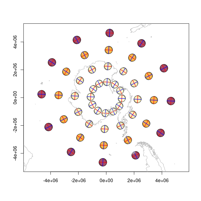

Tissot indicatrixes for a polar stereographic projection using a regular lon/lat input grid, showing unevenly spaced and heavily distorted ellipses that illustrate the problem with lon/lat sampling in a polar projection

plot of chunk polar

la <- tissot(polar_xy, "+proj=laea +lat_0=-90 +lon_0=147")
plot(indicatrix(la), scale = 2.5e5, add = FALSE)
tissot_map()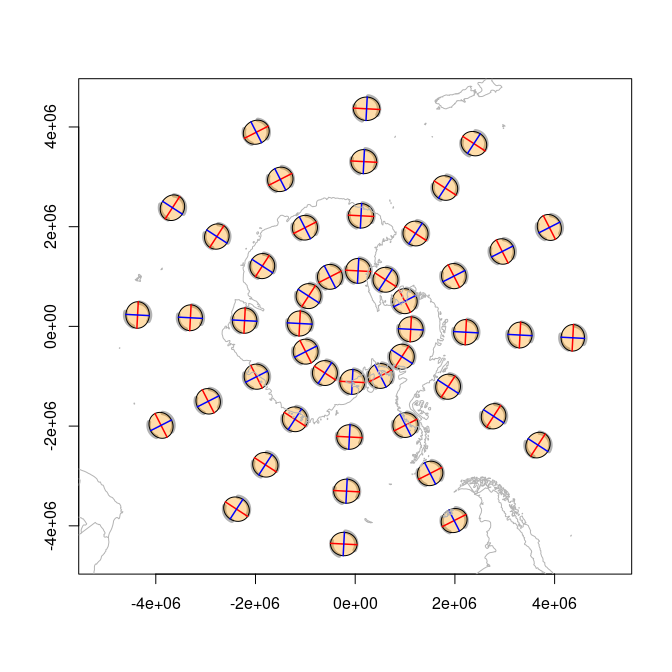

Tissot indicatrixes for a polar Lambert Azimuthal Equal Area projection using a regular lon/lat input grid, showing consistent ellipse areas but irregular spacing near the pole

plot of chunk laea

If we push the centre away from the pole in Azimuthal Equidistant, it’s useful to see what happens.

lea <- tissot(polar_xy, "+proj=aeqd +lat_0=-20 +lon_0=147")
plot(indicatrix(lea), scale = 2.5e5, add = FALSE)
tissot_map()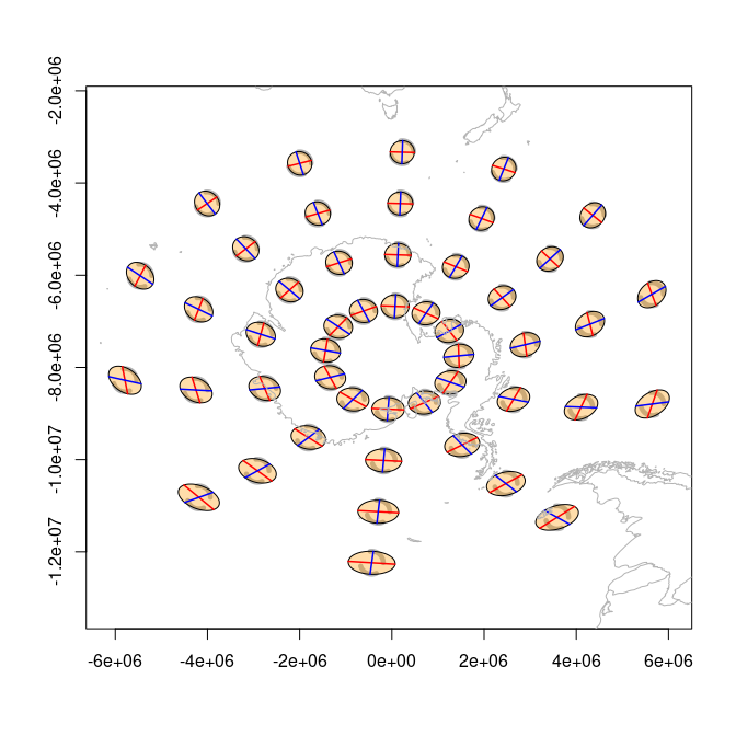

Tissot indicatrixes for an Azimuthal Equidistant projection centred at 20°S, applied to a polar-region lon/lat grid, showing the distortion pattern that results from an off-pole projection centre

plot of chunk aeqd

Consider generating input in the crs you are assessing

As with the UTM example above, using tissot_unproject() it is usually far better to generate a grid in the CRS being assessed. A grid in lon/lat won’t be very meaningful in many projections.

op <- par(mfrow = c(1, 2))
ext <- c(-180, 150, -80, -50)
crs <- "+proj=stere +lat_0=-90 +lon_0=147"

projext <- reproj::reproj_extent(ext, crs, source = "EPSG:4326")
polar <- expand.grid(seq(projext[1L], projext[2L], by = 30 * 1e5), seq(projext[3L], projext[4L], by = 10 * 1e5))
polar_xy <- tissot_unproject(polar, "EPSG:4326", source = crs)
p <- tissot(polar_xy, crs, source = "EPSG:4326")
plot(indicatrix(p), scale = 2.5e5, add = FALSE, fill.by = "scale_area")
tissot_map()

ext <- c(-180, 150, -80, -50)
crs <- "+proj=laea +lat_0=-90 +lon_0=147"
projext <- reproj::reproj_extent(ext, crs, source = "EPSG:4326")

polar <- expand.grid(seq(projext[1L], projext[2L], by = 30 * 1e5), seq(projext[3L], projext[4L], by = 10 * 1e5))
polar_xy <- tissot_unproject(polar, "EPSG:4326", source = crs)
p <- tissot(polar_xy, crs, source = "EPSG:4326")
plot(indicatrix(p), scale = 2.5e5, add = FALSE, fill.by = "scale_area")
tissot_map()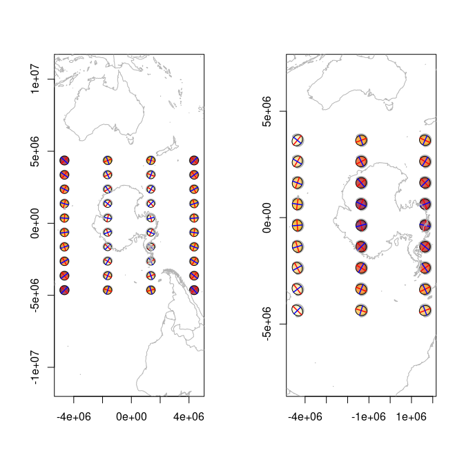

Side-by-side Tissot indicatrix plots comparing polar stereographic and Lambert Azimuthal Equal Area projections, both sampled on a regular grid in projected coordinates, showing much more regular and interpretable distortion patterns than a lon/lat grid

plot of chunk polar-proj

par(op)

Why this package?

Most “Tissot indicatrix” plots you’ll find online are just geographic circles drawn on the map. They show what happens to a circle under the projection, which is useful — but it’s not the indicatrix. The indicatrix is the Jacobian of the projection at a point: it gives you actual scale factors, angular deformation, and areal distortion. This package computes those.

Other examples: mgimond.

Code of Conduct

Please note that the tissot project is released with a Contributor Code of Conduct. By contributing to this project, you agree to abide by its terms.