2 Two questions
2.1 Question one: how are positions worked out from the index?
Every gridded dataset is an array, and every cell has an index: a row and a column, or more generally one integer per dimension. The first question is how much information you need, beyond the index, to say where each cell is.
There is a well established ladder for this, used in scientific visualisation (the VTK data model has a class for each rung) and in Earth system modelling (ESMF, following Balaji’s grid standards work). Each rung relaxes one constraint and needs more stored information than the one before.
Regular. Positions follow from the index by arithmetic alone. The grid is specified by its dimension and an origin and step in each direction, or equivalently by its dimension and extent. That is six numbers for a 2D grid:
ncol, nrow, xmin, xmax, ymin, ymaxThe GDAL geotransform is the same information arranged as an affine transform (origin, step and two shear terms that are zero for an axis-aligned grid). Writing the cell centres out as coordinate vectors adds no information; they are derived values.
Rectilinear. Rows and columns are still straight and at right angles, but spacing varies along each axis independently. The grid needs one vector of positions per axis: nx + ny values. Every cell is at (x[i], y[j]), the outer product of two 1D sequences. Pressure levels, stretched ocean model grids and some reanalysis products are rectilinear in this sense.
Curvilinear. Cells are still indexed by row and column, and each still has four neighbours, but their positions cannot be written as an outer product of two sequences. The grid needs a position per cell for each coordinate: 2 * nx * ny values for a 2D grid.
Unstructured. There is no row and column index at all. Cells are numbered, and which cells neighbour which must be stored explicitly. Triangular meshes, hexagonal MPAS grids and point clouds are unstructured.
| Type | Positions | Stored | CF signal |
|---|---|---|---|
| Regular | implicit, origin plus step | 6 numbers | 1D coordinates, uniform spacing |
| Rectilinear | outer product of two 1D sequences | nx + ny values | 1D coordinates, varying spacing |
| Curvilinear | explicit per cell, still indexed by (i, j) | 2 nx ny values | 2D auxiliary coordinates |
| Unstructured | explicit per cell plus connectivity | positions and topology | UGRID |
The first three rungs are what Balaji calls logically rectangular: in index space every cell is a box. His phrasing is worth keeping: “The coordinate space may continue to be physically curvilinear; yet, in index space, grid cells will be rectilinear boxes.” The containment is strict. Every regular grid is rectilinear, and every rectilinear grid could be stored as curvilinear, wastefully.
2.2 Question two: in which frame?
The ladder says nothing about what the positions are. They have to be numbers in some coordinate frame, and there are several kinds:
- Geographic longitude and latitude, on some model of the Earth.
- Projected coordinates, usually metres (sometimes kilometres), defined by a projection family, a centre, a few parameters and an Earth model.
- Rotated longitude and latitude. Angular coordinates on a sphere whose pole has been moved, as CF’s
rotated_latitude_longitudeand PROJ’sob_tran. These look like longitude and latitude, and are measured in degrees, but they are not geographic. - Projected but angular. The GOES geostationary fixed grid stores
xandyas scan angles in radians. Multiplied by the satellite height they become metres in PROJ’sgeosprojection. - No frame. Index space only: row and column numbers, or the unit square some plotting functions assume.
2.3 The answer to one depends on the other
Here is the point of the book. The first question has no answer until the second is fixed. A grid is regular, rectilinear or curvilinear in a frame, and the same cells give different answers in different frames:
| Grid | In its native frame | In geographic longitude and latitude |
|---|---|---|
| NSIDC 25 km south, EPSG:3412 | regular | curvilinear |
| CORDEX rotated-pole model grid | regular (rotated longitude/latitude) | curvilinear |
| AVISO global Mercator | regular (Mercator) | rectilinear |
| GOES ABI full disk | regular (scan angle, or geos metres) |
curvilinear, partly undefined |
| OISST quarter degree | regular (longitude/latitude) | regular |
| MODIS land tile (SIN grid) | regular (sinusoidal) | curvilinear |
| NEMO ORCA tripolar | curvilinear | curvilinear |
| VIIRS level 2 swath | curvilinear | curvilinear |
Only the last two rows are curvilinear in every frame. They are what people should mean by “curvilinear”, and they are a minority of the grids that get the label.
Two consequences follow, and both come back repeatedly.
“Curvilinear” without a frame is underspecified. A grid that is curvilinear in longitude and latitude may be regular in some other frame. The useful statement is “regular in EPSG:3412” or “curvilinear in every frame we tried”.
“Longitude and latitude” says nothing about regularity. OISST is regular in longitude and latitude. A rotated-pole grid is regular in a longitude and latitude frame too, just not the geographic one. Being in degrees does not make a grid curvilinear, and being curvilinear does not make it geographic.
2.4 A third thing: storage
There is one more layer, and it is where most of the confusion lives. What a file stores is a choice made by its producer, and it does not have to match the grid’s real structure. A regular grid can be stored as six numbers, as two coordinate vectors, or as two full 2D arrays, in its own frame or in another. Conventions like CF read the grid type from the shape of the stored coordinate arrays, so the storage choice becomes the label.
Chapter 3 lists those storage forms. The short version: the ladder describes geometry, the frame describes what the numbers mean, and storage describes what the producer wrote down. Three different things, routinely collapsed into one word.
2.5 Things that are not part of either question
Several nearby issues are real and important, but they are separate from the two questions, and mixing them in makes the picture harder to see.
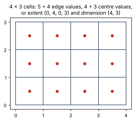
- Cell semantics. Do coordinates refer to cell centres or corners (GeoTIFF’s PixelIsPoint and PixelIsArea)? Are there
ncoordinates orn + 1edges? Are there CFboundsarrays? This is the half-pixel problem, and it exists on every rung of the ladder (Figure 2.1).
- Numeric precision. Coordinates stored as 32-bit floats carry noise. Whether a grid is “regular” is always a question with a tolerance.
- The shape of the Earth. The ladder is deliberately silent about the manifold. A regular longitude and latitude grid’s left and right edges are the same meridian and its top row is one point, and nothing in the grid structure says so. That is a feature of the ladder, not a gap, and Chapter 8 returns to it.
- The word “dimension”. In array software a dimension is an axis.
lon(y, x)is one 2D coordinate variable on two dimensions. It does not add dimensions. Coordinate dimension and topological dimension are different again; the trianglewins note “On dimension” covers those.