8 Edges of the map
The two questions in this book are about index structure and frame. They deliberately say nothing about the surface the data describes. This last chapter is about where that silence matters, and what lies past it.
8.1 The ladder does not know about the sphere
A regular 1 degree longitude and latitude grid has 360 by 180 cells. By the ladder it is as regular as a grid can be. But its top row is 360 cells that all touch one point, the pole. Column 0 and column 359 are neighbours across the antimeridian and as far apart as possible in index space. None of this is encoded in the grid; it is knowledge the application must supply.
That is not a failure of the ladder. Regularity is a property of the indexing, not of the surface, which is why the same ladder works on a plane, a sphere or a torus. The longitude and latitude case simply shows what happens when you discretise a sphere with a tool designed for a rectangle: the grid is correct, and the mismatch is between the grid’s scope and the application’s needs.
8.2 Workarounds that stay on the ladder
Most geoscience stays on the ladder and handles the sphere by convention:
- Tripolar ocean grids move the singular points onto land. The topology lives in the coordinate arrays and the model’s halo exchange, not in the index.
- Polar projected grids such as the NSIDC grids put the pole in the middle of a regular grid. The antimeridian becomes an ordinary line through the interior.
- Choosing the frame for the problem. A polygon that crosses the antimeridian is only awkward in longitude and latitude. Warp the grid to a frame where the region is compact, do the work there, and the problem goes away. The OISST example in Section 7.8 is the statistical version of the same move.
Grid arithmetic libraries such as vaster and vapour are deliberately silent about topology. That is the right scope: sphere topology belongs in a layer above grid indexing.
8.3 The binned grid: the smallest step off the ladder
NASA’s Ocean Biology Processing Group bins level 3 ocean colour data with the Integerized Sinusoidal Binning Scheme, published with SeaWiFS (Campbell, Blaisdell and Darzi 1995) and used since for CZCS, OCTS, MODIS, VIIRS, MERIS, Aquarius and PACE. It is worth a section of its own because it is the simplest grid that takes the sphere seriously, and because it breaks the ladder in an instructive way.
The rules fit in a few lines:
- the globe is split into
NUMROWSzonal rows of equal latitude height (an even number, so no row straddles the equator); - each row is divided into a whole number of equal bins, proportional to the cosine of the row’s central latitude;
- bins are numbered from 1, south to north, and west to east from the 180 degree meridian within each row;
- each polar row ends up with exactly 3 bins.
As arithmetic:
latbin[row] = (row + 0.5) * 180 / NUMROWS - 90          # row = 0 .. NUMROWS - 1
numbin[row] = int(2 * NUMROWS * cos(latbin[row]) + 0.5)
basebin[row] = 1 + sum(numbin[0 .. row - 1])
row  = int((90 + lat) * NUMROWS / 180)
bin  = basebin[row] + int((lon + 180) * numbin[row] / 360)
lon = 360 * (bin - basebin[row] + 0.5) / numbin[row] - 180scripts/make_figures.py.
| NUMROWS | Bin size | Total bins | Used for |
|---|---|---|---|
| 180 | 1 degree, about 111 km | 41,252 | Aquarius |
| 2160 | 5 minutes, about 9.28 km | 5,940,422 | SeaWiFS, OCTS |
| 4320 | 2.5 minutes, about 4.64 km | 23,761,676 | MODIS, VIIRS, MERIS, CZCS |
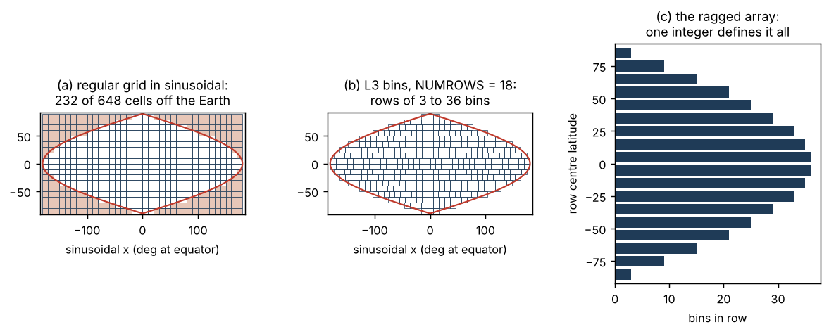
Why ragged. The sinusoidal projection is equal area, so a regular grid in it has equal-area cells, but the Earth occupies only the lens-shaped middle of the rectangle (Figure 8.1 a). Forcing a sphere into that rectangle leaves about 36% of the cells empty by construction. The binning scheme keeps the equal-area idea and drops the rectangle: each row gets as many bins as its latitude band needs (Figure 8.1 b). The result is a ragged array, not a matrix.
Where it sits on the ladder. By the ladder’s definitions this is unstructured: there is no global (i, j) index, only a bin number. But it is nothing like a mesh. Every bin’s position follows from its number by arithmetic, and the entire global scheme is defined by one integer, NUMROWS, the way a regular grid is defined by six numbers. So L3 bins break the usual pairing on the ladder, where implicit positions go with structured indexing and explicit positions with unstructured. They are implicit and unstructured. That combination is what discrete global grid systems are built on, which is why the scheme reads well as the simplest possible DGGS.
What files store. Because the addressing is implicit, a binned file stores only the bins that have data: a list of bin numbers with their statistics (observation counts, weights, sums), and a per-row index into that list. Coordinates are never stored; they are computed from the bin number when needed. That is the entropy argument of Chapter 3 taken to its conclusion.
Its limits as a DGGS. It is the simplest, not the best:
- Nearly equal area. Rounding each row to a whole number of bins makes bin areas vary by about 7% from smallest to largest, at all three standard resolutions.
- Not hierarchical. Doubling
NUMROWSdoes not split each bin into four; from 2160 to 4320 rows, only about 11% of child rows have exactly twice their parent’s bins. - Bins are longitude and latitude rectangles, so their shape degrades toward the poles, and the 180 degree meridian is still a seam.
- Neighbours in the next row are found by arithmetic on longitudes, not by a fixed offset.
- With 32-bit bin numbers the scheme overflows at about 41,000 rows (roughly 500 m bins). Precision bites earlier: the OBPG page warns that 32-bit and 64-bit arithmetic can put the same coordinates in different bins at the finer resolutions.
- Bins are laid out on a sphere (radius 6378.145 km), not the ellipsoid, which adds its own small departure from equal area.
H3, S2 and HEALPix trade more complicated addressing for hierarchy and better cell shapes. L3 bins show what the first step away from the rectangle looks like.
Tools and references. The R package hypertidy/L3bin (github.com/hypertidy/L3bin) implements the scheme without materialising it: L3bin(NUMROWS) returns the row tables, and bin_from_lonlat(), lonlat_from_bin(), extent_from_bin() and crop_bins() work from those.
library(L3bin)
L3bin(2160)$totbins                 # 5940422
bin_from_lonlat(147, -42, 2160)     # the bin containing Hobart
lonlat_from_bin(c(1, 2, 3), 2160)   # the three bins of the south polar row
The OBPG format page, Integerized Sinusoidal Binning Scheme for Level 3 Data (oceancolor.gsfc.nasa.gov/resources/docs/format/l3bins/; archived at web.archive.org, snapshot 6 January 2026), gives the rules, the resolution table and reference Perl routines (initbin, latlon2bin, bin2latlon, bin2bounds); its Figure 1 uses the same 18 rows of 10-degree bins as Figure 8.1. The original description is NASA Technical Memorandum 104566, Volume 32. An ASCII Markdown copy of the page, made from the archived snapshot, is kept with this project’s files (l3bins-archive/).
8.3.1 Two things called “sinusoidal”
The word “sinusoidal” names two very different grids in NASA data, and moving between them crosses the whole map of this book.
- The ocean colour bins above: a ragged array, unstructured but implicit, defined by
NUMROWS. No CRS is needed to compute a bin’s position; the scheme is “sinusoidal” only in the sense that row lengths follow the cosine of latitude. - The MODIS land tiles (the “SIN grid”): a regular grid in a projected CRS,
+proj=sinu +R=6371007.181. The world is cut into 36 by 18 tiles of 10 degrees at the equator, 1,111,950.52 m on a side, and each tile is a regular raster: 2400 by 2400 cells of 463.31 m for the 500 m products, 4800 of 231.66 m for 250 m, 1200 of 926.63 m for 1 km. Tile and cell positions are six numbers in that CRS, and GDAL reads them as an ordinary geotransform.
The second is the regular sinusoidal grid of Figure 8.1 a: equal area, and with a large share of its cells outside the Earth, which is why tiles that are entirely off the Earth or entirely ocean are simply not produced. In longitude and latitude its meridians lean further from vertical with distance from the central meridian, so a MODIS tile written out as longitude and latitude arrays looks curvilinear, exactly like the NSIDC grid in Figure 1.1. And the ocean colour mapped products (standard mapped images, SMI) are a third grid again: the bins interpolated onto a regular longitude and latitude raster. At the equator an SMI pixel matches a bin exactly; toward the poles there are more and more SMI pixels per bin, so the regular raster repeats information the bins held once.
So the same instrument’s data can arrive as a ragged equal-area index, a regular sinusoidal raster, or a regular longitude and latitude raster, and a reader who only hears “sinusoidal” cannot tell the first two apart. In the two-question terms: the bins have no frame and no (i, j) index at all; the land tiles are regular in a sinusoidal frame; the mapped images are regular in longitude and latitude.
8.4 Discrete global grid systems
Discrete global grid systems (H3, S2, HEALPix, ISEA) go the whole way. The sphere comes first, and adjacency, area and hierarchy are correct by construction. The price is the global row and column index. They sit outside the ladder not because they are more complicated, but because they answer a different question: what is the right cell scheme for a sphere, rather than how is this array positioned.
8.5 Meshes and the word “dimension”
The same conflation appears in meshes. Triangulating longitude and latitude as planar x and y gives the right topology (which triangle touches which) and the wrong geometry: areas and angles are in degrees, distorted toward the poles, and the Delaunay property holds on the plane, not on the sphere. That is the mesh version of treating a frame as if it were geometry. The trianglewins note “On dimension” takes this up, along with the separate confusion between coordinate dimension (how many coordinates each vertex has) and topological dimension (what kind of shape it is). In array software, “dimension” means a third thing again: an axis. A grid with lon(y, x) has two dimensions, whatever its coordinates.
8.6 The question to carry away
Every grid in this book can be described by two short answers: how positions follow from the index, and in which frame. Most of the grids called curvilinear are regular in a frame someone forgot to write down. Before you regrid, resample or reach for the 2D arrays, ask the title question: regular in what?