3  One grid, many costumes

3.1 Ten ways to store the same thing

A regular grid can arrive in many forms, depending on what its producer chose to write down. Some of these are genuinely different structures. Others are the same information in a more expensive encoding. The earliest version of this list (the rw-book draft) had eight cases labelled A to H; two more are added here, because without them the frame question stays hidden.

Table 3.1: Storage forms of a grid, with what is underneath.

	What is stored	Real geometry	Example	Common label
A	an array, no position information	unknown	a PNG, a raw binary	non-georeferenced
B	dimension plus affine transform (and CRS)	regular	GeoTIFF, COG	regular
C	1D coordinate vectors, uniform spacing	regular	OISST, ERA5, GHRSST	rectilinear (“degenerate rectilinear”)
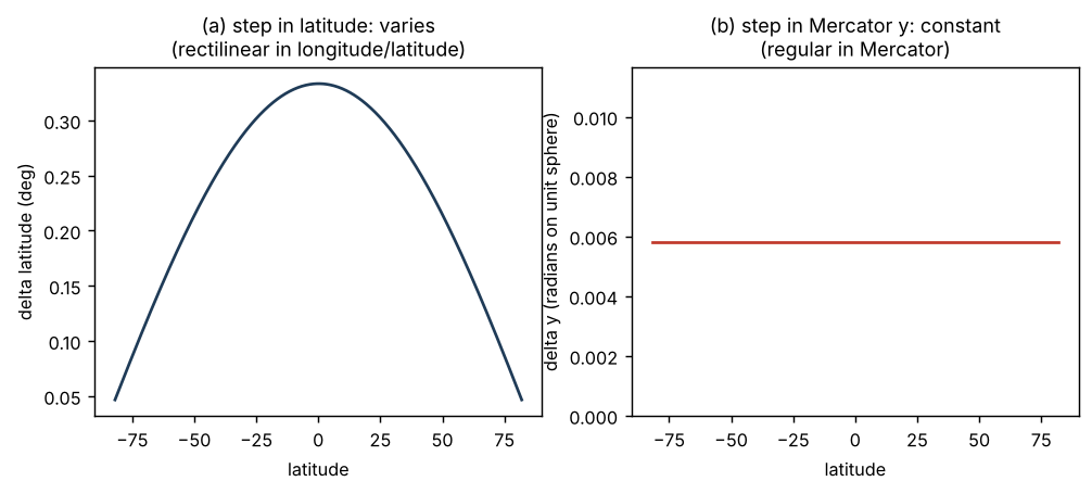
D	1D longitude and latitude vectors, latitude spacing varies	regular in Mercator	AVISO altimetry	rectilinear
E	2D longitude and latitude arrays	regular in a projection	CryoSat-2 on EPSG:3412; CORDEX HCLIM and MAR	curvilinear (“cryptic curvilinear”)
E2	2D longitude and latitude arrays, plus rotated 1D axes	regular in rotated longitude/latitude	CORDEX RACMO	curvilinear
E3	1D scan-angle vectors, CRS not carried	regular in geos	GOES ABI in a Zarr store	regular, frame unknown
F	2D arrays of native projected x and y	regular in that projection	rare	curvilinear
G	1D coordinate vectors, spacing genuinely varies	rectilinear	pressure levels, stretched grids	rectilinear
H	2D coordinates, regular in no frame	curvilinear	NEMO ORCA, VIIRS swath	curvilinear

Only G and H store information that could not be recovered from six numbers and a frame. Everything from C to F is a regular grid in costume.

The labels in the last column are what conventions and software would call each case, judging from the stored arrays. They are wrong for C to F. Two of those mislabellings are common enough to have names.

3.2 Degenerate rectilinear

Case C is the netCDF default. A regular longitude and latitude grid is written with a 1D coordinate variable for each axis, one value per cell centre. The format allows the spacing to vary, which makes this rectilinear storage, but the values are evenly spaced, so the grid is regular. The term used for this on hypertidy.org since 2022 is degenerate rectilinear: a rectilinear container carrying regular content.

This is mostly harmless, because a reader can test the spacing and recover the six numbers. It becomes a problem in two ways.

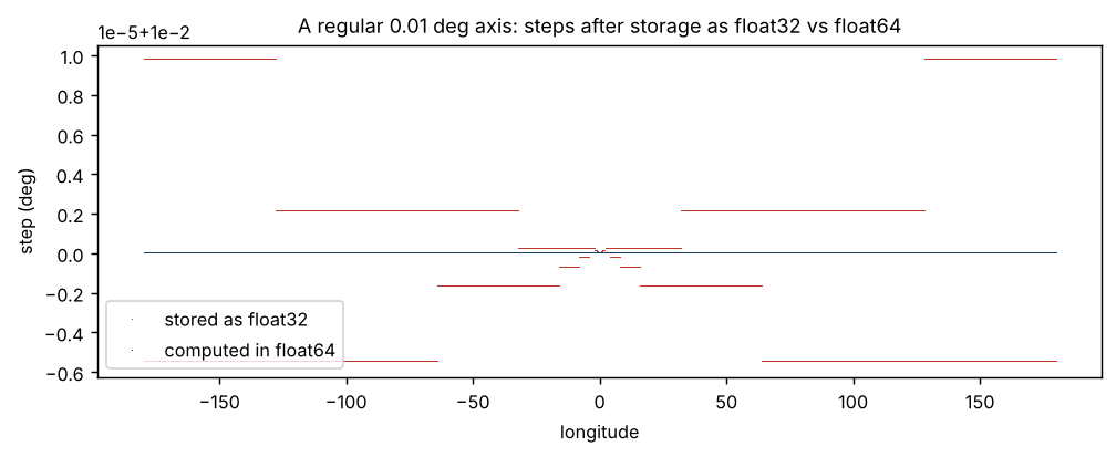
First, the spacing test needs a tolerance, and 32-bit storage makes the tolerance matter. Figure 3.1 shows a regular 0.01 degree longitude axis, like the one in the MUR GHRSST product (36000 columns). Computed in 64-bit floating point, the steps vary by about 6e-14 degrees. Stored as 32-bit floats, they vary between 0.0099945 and 0.0100098, a spread of about 0.15% of a cell. A test that asks whether every step is exactly equal says this grid is irregular. It is not.

Figure 3.1: Steps between successive values of a regular 0.01 degree longitude axis, when the values are held in 64-bit (dark) and 32-bit (red) floating point.

Second, the stored values may not even describe the intended grid precisely. The GHRSST MUR files store 36000 longitudes and 17999 latitudes; their longitude values are aligned to the right edge rather than centred, there is a missing half-row at each pole, and the metadata claims a range of -180 to 180 and -90 to 90 that the coordinates do not match. The six numbers have to be decided by a person; the arrays only suggest them (Section 7.3).

3.3 Hidden projections

Case D is subtler. The AVISO global altimetry products were computed on a Mercator grid: regular in Mercator x and y. They were distributed with 1D longitude and latitude vectors. Longitude is still evenly spaced, because Mercator x is proportional to longitude, but latitude is not, because Mercator y stretches toward the poles. The file therefore looks like a genuinely rectilinear grid with variable latitude spacing (case G).

Figure 3.2: A Mercator grid with 1/3 degree longitude spacing, 915 rows. (a) The latitude steps vary from 0.33 degrees at the equator to under 0.05 at 82 degrees. (b) Converted back to Mercator y, every step is the same to within 2e-15.

Figure 3.2 shows the test that reveals it. Convert latitude to Mercator y and the steps become constant to machine precision. The gproj detection on a real AVISO file found a deviation of 1e-12. That is not a coincidence or an approximation; the coordinates were computed from the formula.

Case E is the same story with both axes. A grid that is regular in a projection, written out as longitude and latitude for every cell, becomes 2D coordinate arrays. CF reads 2D auxiliary coordinates as a curvilinear grid, and so does nearly every tool built on CF. The name for this used on hypertidy.org is cryptic curvilinear: a grid that presents as curvilinear but is regular in a frame the file has forgotten.

Cases E2 and E3 are the same pattern in frames that are easy to overlook. A rotated-pole climate model grid is regular in rotated longitude and latitude. Well-made files carry both the rotated 1D axes and the 2D geographic arrays; some readers prefer the 2D arrays and see a curvilinear grid (Section 7.4). A GOES full disk image is regular in scan angle; if the projection variable is lost in conversion, the 1D coordinates survive but nobody downstream knows what they measure (Section 7.5).

3.4 The entropy argument

Why care, if the arrays are correct? Because they are a strictly worse encoding of the same grid.

Figure 3.3: Values stored to describe one grid, under three encodings. Log scale.

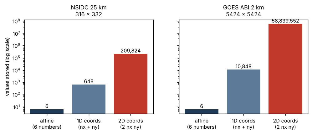
• More data. Figure 3.3 shows the counts. For the NSIDC grid, six numbers become 648 as coordinate vectors or 209,824 as 2D arrays. For GOES at 2 km, six become 10,848 or 58,839,552.
• Less precision. The six numbers are exact. Derived coordinates carry rounding from the projection maths and from storage, so the expensive encoding is also the noisier one.
• Less meaning. Six numbers and a CRS let any reader compute distances, areas and neighbourhoods in the native frame. Arrays of longitude and latitude do not say which frame was native.
• More work downstream. A regular grid can be subset, aligned and warped with index arithmetic. A curvilinear one needs search structures and interpolation.

The general rule for producers follows directly: if the grid is regular in some frame, store the frame and the six numbers. Coordinate arrays are fine as a convenience alongside them, never instead of them.

3.5 The other side

It would be wrong to finish this chapter suggesting coordinate arrays are a mistake. For cases G and H they are the only correct description. A tripolar ocean grid cannot be written as six numbers in any frame; its 2D arrays are the grid. A satellite swath follows the scan geometry of an instrument, and its geolocation arrays are what the instrument measured. The climate modelling community’s habit of treating coordinate arrays as the complete description of a grid is exactly right for its own models, which is why that habit is so strong. The next chapter is about those habits, and why reasonable people end up seeing the same file differently.